Introduction to CityJSON
Paulo Raposo
pauloj.raposo@outlook.com
2023-03-13.
© Paulo Raposo, 2023. Free to share and use under Creative Commons Attribution 4.0 International license (CC BY 4.0).

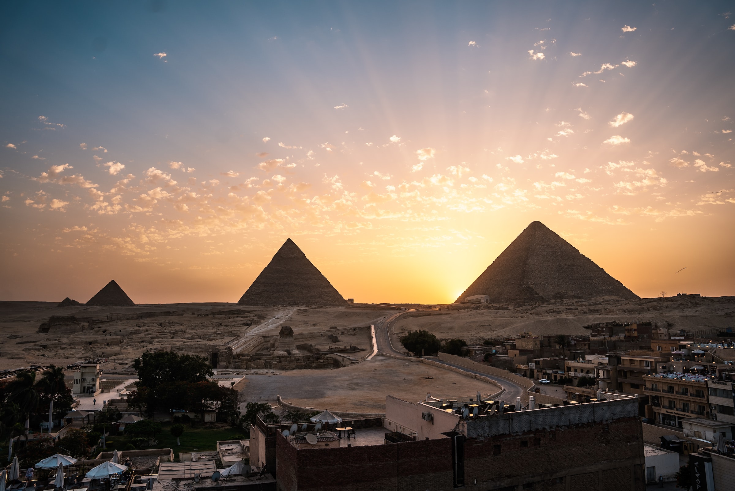 Image by Ruben Hanssen, from Unsplash.
Introduction
Geographic Information Systems (GIS) have usually been very two-dimensional, but they're getting more and more 3D. In this tutorial we'll get to know a recently-invented, 3D data format designed to model buildings, bridges, and other structures: CityJSON. It's an official Open Geospatial Consortium (OGC) standard, and interoperates with CityGML, another such standard. CityJSON is maintained by, among others, the folks at TU Delft's 3D Geoinformation research group. Its essentially an application of Javascript Object Notation (JSON), tailored to handle 3D vector geometry, geographic coordinate systems, and GIS-style object attributes. And it's free and open-source!
To get well acquianted with CityJSON, we're going to write up a data file from scratch. That's not normally how one would interact with a CityJSON file, as they're typically very long text files in practice, storing perhaps thousands of buildings and many thousands of geometric points: various software packages, including several offered by the CityJSON team themselves, can load, edit, and write CityJSON (and other related 3D geometry files) in an interactive or programmatic manner. But this tutorial will build a very short example with just one, simple building, so that we can keep track of all the essential parts in our learning.
And we'll learn this new file format by modeling a very old building!
Plotting out The Great Pyramid of Cheops (Khufu)
This ancient Egyptian pyramid makes a good subject for building a basic model from scratch, since we can define the overall shape using just five points in 3D space. Let's get coordinates using Open Street Map. At openstreetmap.org, head over to Giza, Egypt, where the famous three pyramids stand. We'll model the largest one, the Great Pyramid of Cheops (Khufu), which is the one that stands the furthest north-east.
We need the latitude and longitude coordinates of 5 points to make our simple pyramid model: the four ground corners and the pinnacle in the center. Get these coordinates using the Open Street Map site by carefully placing your cursor on each one and right clicking:
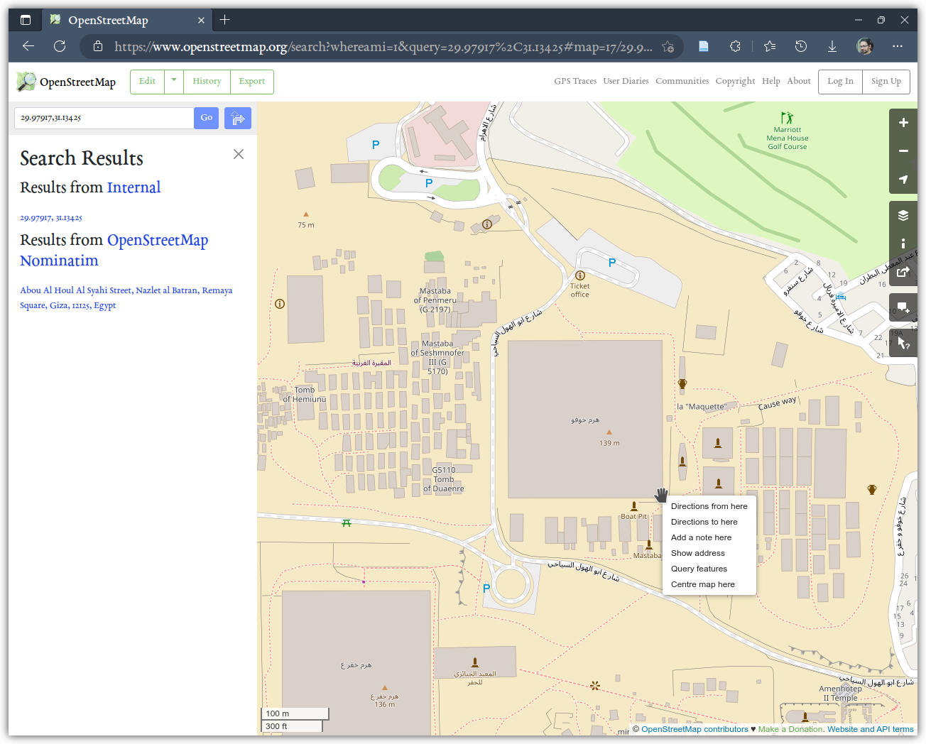
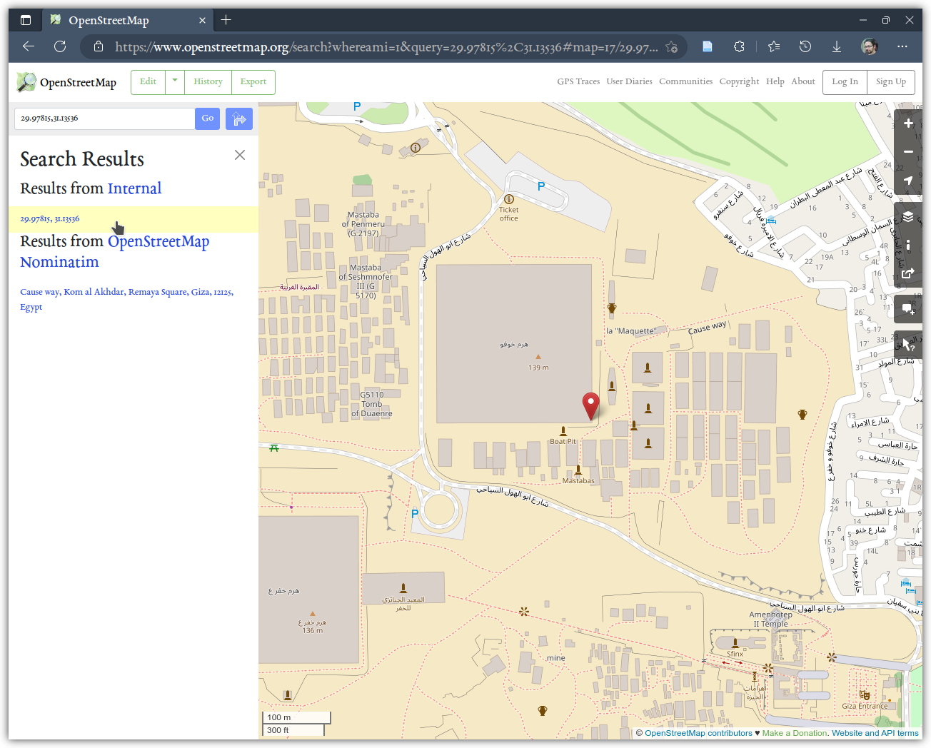
Select "Show address," and the left part of the page will give you latitude and longitude coordinates for the spot you clicked over:
Jot down the values for all five coordinates, and, for the purposes of this tutorial, don't worry about being super precise about exactly what position you clicked on or exactly what number you get. Here are the points I got, with longitude and latitude pairs written in blue, and with counter-clockwise index numbers starting at zero in red:
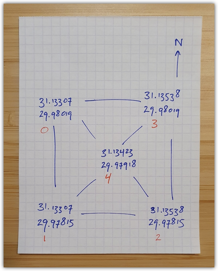
Here they are in index sequence and in (x,y) order (as opposed to the more commonly geographic y-latitude, x-longitude order that OSM reported them in):
31.13307,29.98019
31.13307,29.97815
31.13538,29.97815
31.13538,29.98019
31.13423,29.97918
These are longitude and latitude (i.e., x,y) coordinates, measured in degrees, the WGS 1984 coordinate system that OSM is using. In a 3D model we'll need a third, z coordinate to represent height, and having that coordinate in degrees is a bad idea, because that doesn't make much geometric sense. So we're going to project our WGS 84 coordinates into a map projection that uses meters as its unit of measure. A good one to choose that covers the pyramid is the UTM zone 36 North.
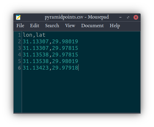
Now, the math involved to convert these coordinates can be a little daunting to do by hand, or to type out into a program. But we can let our trusty friend QGIS do this for us. Put those coordinates in a CSV file that looks like this (I'm calling mine pyramidpoints.csv):
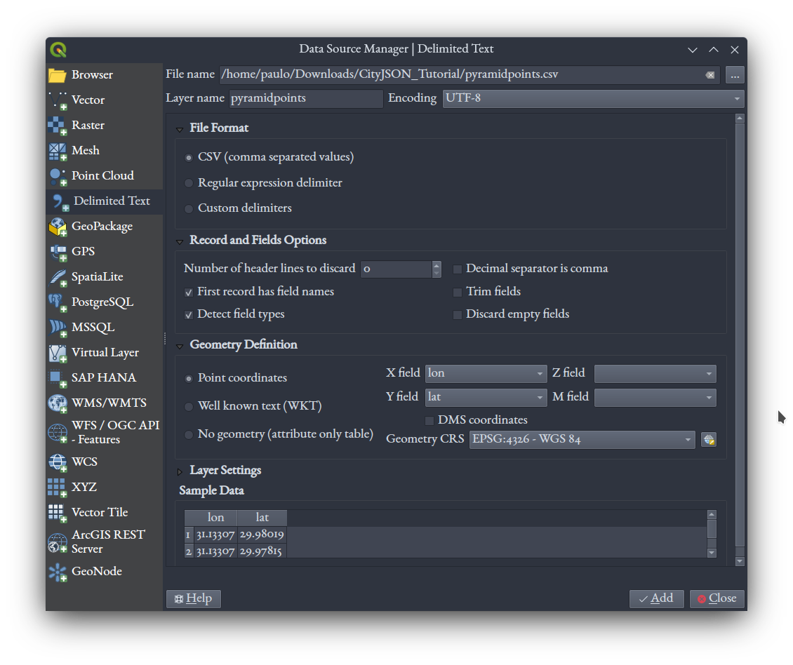
Fire up QGIS, and load that file using the "Delimited Text" tab in the Data Source Manager.
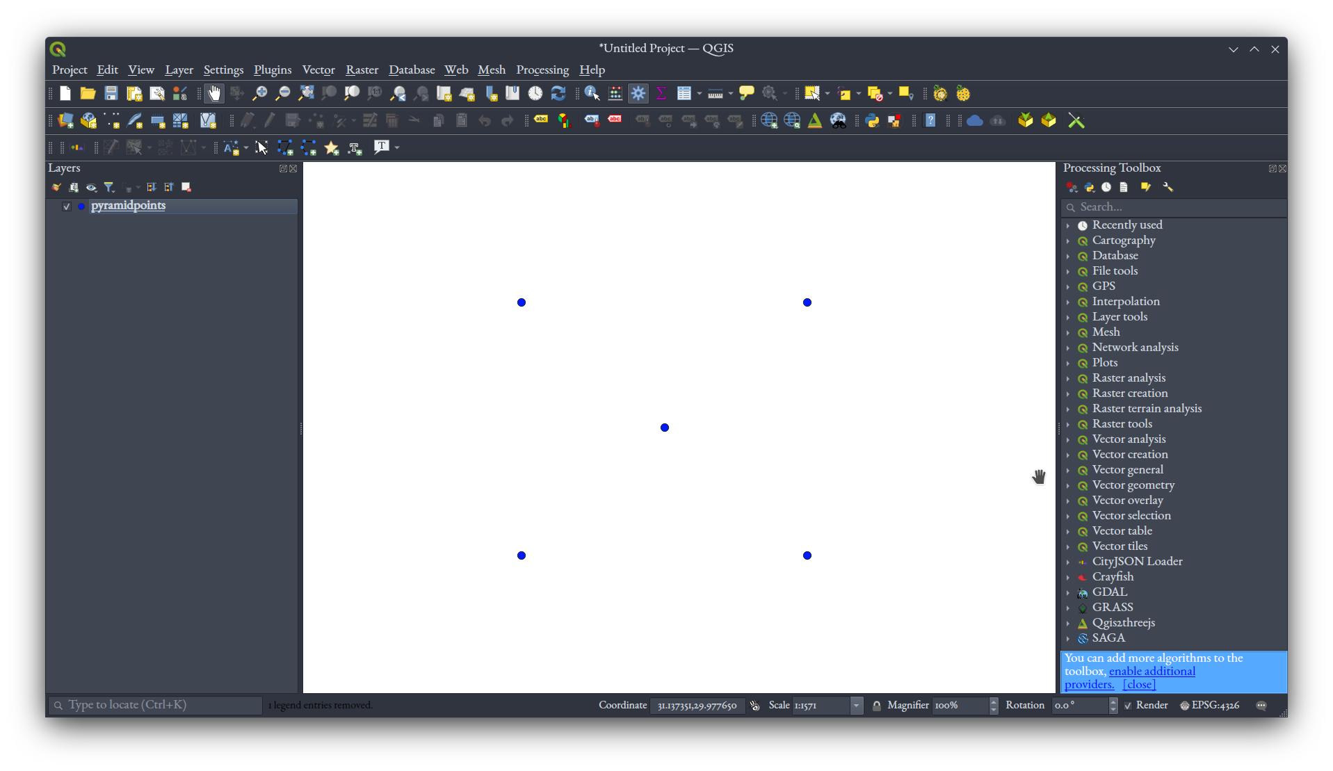
You should get something pretty square, just like we expect:
To get a little extra confidence we've placed things right, let's add an aerial image layer underneath. Again in the Data Source Manager, select the XYZ tab, and add a new source for Bing Aerial tiles, using this URL:
http://ecn.t3.tiles.virtualearth.net/tiles/a{q}.jpeg?g=1
Adding that layer with the pyramid points on top will give you:
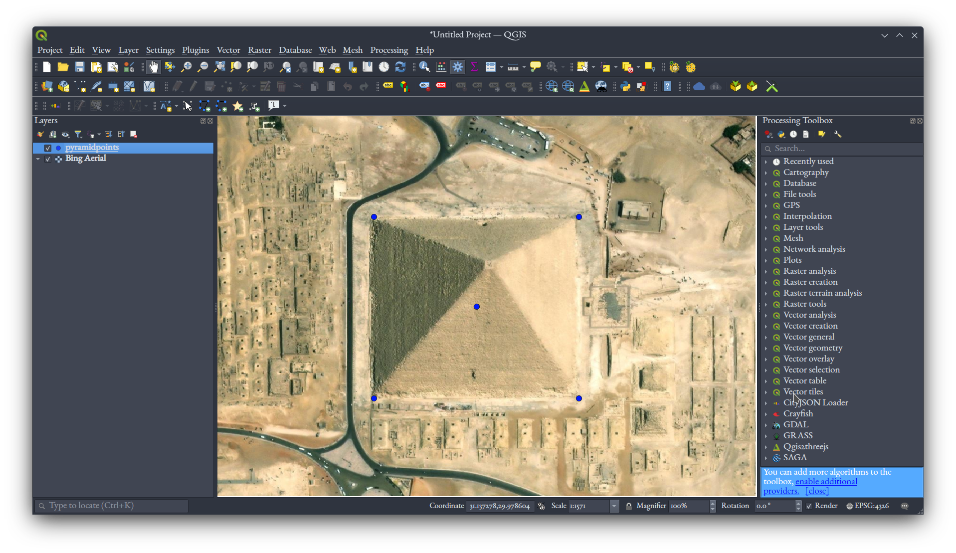
Notice that the pinnacle point doesn't line up with the pinnacle in the image! That's due to the imperfection of georectified imagery, not to the location we clicked for our point. Notice in the image that the north face of the pyramid seems smaller than the south, but that's not true in reality - it's just perspective at play in the photography.
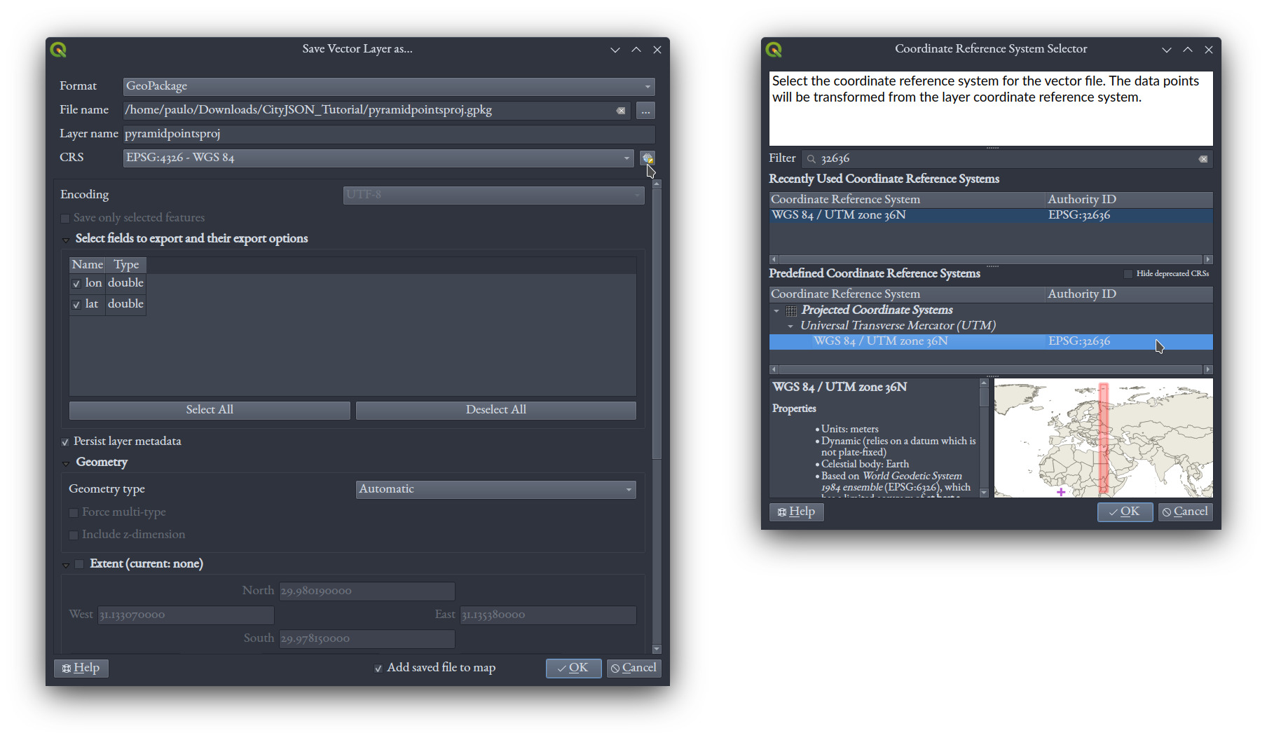
Right-click on the points layer in the Layers panel, and choose Export, Save Features As. Save as a GeoPackage, with a new name (I'm calling mine pyramidpointsproj.gpkg), and importantly, click the little globe/map icon to define a different coordinate reference system (CRS). Search for "32636" to find the UTM zone 36N coordinate reference system (i.e., 32636 is the code by which it's identified in the EPSG system). Select that one.
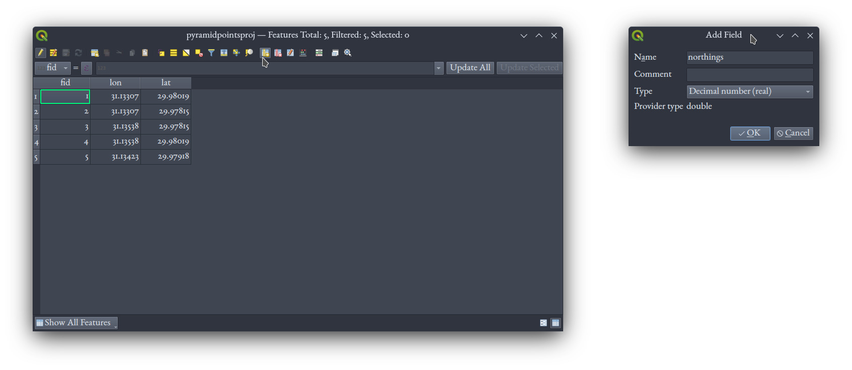
Open the attribute table for the new layer. Click on the little pencil icon to go into "editing mode." Add two new fields, called eastings and northings, respectively, with both of type "Decimal number (real)."
Next, open the Field Calculator, choose to update an existing field, select "eastings," and enter $x as the expression:
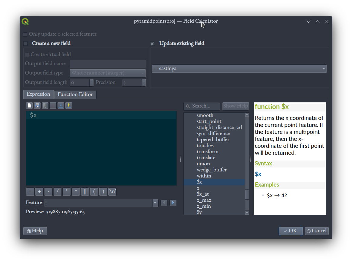
Repeat the same for "northings," but with $y as the expression. You should then have an attribute table that looks like this, including the eastings and northings in meters for the five points:
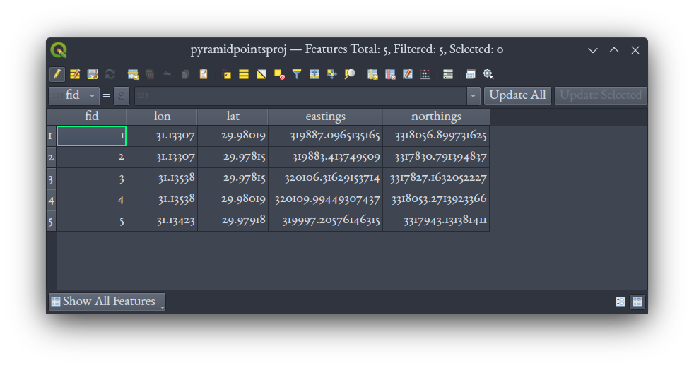
Click the pencil icon to toggle editing off, being sure to save your edits.
Back in the main QGIS window, right-click to Export the GeoPackage layer. Choose CSV as the format and export it. Deleting or disregarding the other columns, you should now have this in your file:
eastings,northings
319887.096513517,3318056.89973162
319883.413749509,3317830.79139484
320106.316291537,3317827.16320522
320109.994493074,3318053.27139234
319997.205761463,3317943.13138141
Now, we're making a 3D model, so we need a third, z coordinate for height. PBS Nova tells us that this pyramid was 146.5 meters tall, before losing some of its pinnacle. So, we'll set each of our four base, corner points' z coordinate to 0.0, and the center, pinnacle one's to 146.5. Also, we've got eastings and northings to a ridiculous number of decimal places, so let's round them down to 1. So our new coordinates table should now look like this, with appropriate headers and a third coordinate, with all three dimensions in meters:
eastings,northings,height
319887.1,3318056.9,0.0
319883.4,3317830.8,0.0
320106.3,3317827.2,0.0
320110.0,3318053.3,0.0
319997.2,3317943.1,146.5
Alright, now we've got all the geometry we need, and in the right coordinate system. Let's start writing some CityJSON!
The CityJSON file
JSON is a very intuitive format for writing all kinds of data. And, as a major benefit, JSON is readable by both humans and machines. The essential concept is that everything is recorded using "objects" described by name and value pairs and "arrays," which are sequenced lists. The name and value pairs use curly brackets, while sequenced lists use square ones. And these two structures can be nested within each other as recursively as necessary. A simple example might be
{
  "People": [
    {"name": "Ophelia", "age": 44},
    {"name": "Bartholomew", "age": 42}
  ]
}
where People is an array that contains two objects, each of which represents a person, storing that person's name and age. Since we can define our objects and arrays any way we like, JSON is very adaptable to all sorts of data. CityJSON has made use of that adaptability to define a standard for 3D geographic vector geometry.
We'll start by laying out the basic skeleton of a CityJSON file (i.e., the "boilerplate" code). Create a new text file called pyramid.json and write the following into it, including some objects and arrays we'll fill in shortly.
{
  "type": "CityJSON",
  "version": "1.1",
  "CityObjects": {},
  "vertices": [],
  "metadata": {},
  "transform": {}
}
First of all, let's deal with the geometry we've worked so hard to get. The points we've defined will go into the vertices object. But, as per the CityJSON format, they need to go in as integer values, not decimal values---that's done to save on file size and complexity, because integers are less expensive to store in computer memory. The CityJSON format still allows for decimal-value coordinates, but it does that by multiplying and adding to coordinate values using a transform, being a set of six numbers that allow the software reading the CityJSON file to convert the integer values back to their correct geographical, decimal number positions. For each of the x, y, and z axes, the transform defines a scaling factor, and a translation value, such that multiplying a coordinate value by the scaling factor increases or decreases it (as well as restoring its decimal number type), and adding the translation value shifts it along that axis by the value.
For our pyramid, we'll conform to the format by multiplying every coordinate we have by 10 (i.e., shifting the decimal place one to the right), and writing that value as an integer (no decimal places). We won't translate, which is mathematically equal as saying we'll translate by 0.0 in every dimension. That means our transform needs to multiply each of the x, y, and z dimensions by 0.1 to get back to our real spatial coordinates, and it needs to add 0.0 to each dimension, too.
Also, we were specific about defining our coordinates in the UTM zone 36N coordinate system. CityJSON allows you to define the coordinate system used in an object called referenceSystem within metadata. It needs to refer to a URL on the opengis.net server, following the format
https://www.opengis.net/def/crs/AUTHORITY/VERSION/CODE
where AUTHORITY needs to be replaced with the organization that defined the coordinate system (this is often "EPSG"), VERSION with the organization's coding version (or zero if there's no version), and CODE with the actual code for the coordinate system. We know our projection is defined by the EPSG with code 32636, and we'll go with version 0.
Our modified 3D points, our transform, and our coordinate reference system thus appear in our CityJSON file now like so:
{
  "type": "CityJSON",
  "version": "1.1",
  "CityObjects": {},
  "vertices": [
    [3198871, 33180569, 0],
    [3198834, 33178308, 0],
    [3201063, 33178272, 0],
    [3201100, 33180533, 0],
    [3199972, 33179431, 1465]
  ],
  "metadata": {
    "referenceSystem": "https://www.opengis.net/def/crs/EPSG/0/32636"
  },
  "transform": {
    "scale": [0.1, 0.1, 0.1],
    "translate": [0.0, 0.0, 0.0]
  }
}
CityJSON works by defining all the coordinates used by features in the file in that vertices list. For each thing in the dataset (e.g., a building), we build it up, surface by surface (e.g., walls) by refering to spatial loops of those vertices. Instead of defining each wall of a building, for example, by restating point coordinate values all the time, CityJSON uses references to the points in the vertices list in terms of where they fall in sequence (remember, vertices is a JSON array, where the order of things listed matters). Using a numbering scheme very common among computer languages, the first point given is in index position 0, the next one at 1, and so on, such that the last point for our data is at index 4. Notice, also, that the x, y, z points are each themselves stored in an array, so that vertices is an array of arrays. CityJSON stores points in the one, centralized vertices array, instead of with each feature in the dataset, to save on file size, since points that are common across features don't have to be restated all the time: two or more features can just refer to the one point. It also helps to implicitly store topological relations, when, for example, two adjacent buildings share some common points where they touch.
Let's build up our pyramid to arrive at our final CityJSON file! We'll call it "pyramid_1" in our data, and it will be one of the CityObjects. So we include it with type, attributes, and geometry properties:
{
  "type": "CityJSON",
  "version": "1.1",
  "CityObjects": {
    "pyramid_1": {
      "type": "Building",
      "attributes": {
        "name": "Great Pyramid of Cheops (Khufu)"
      },
      "geometry": [
        {
          "boundaries": [
            [ [[0, 1, 4]], [[1, 2, 4]], [[2, 3, 4]], [[3, 0, 4]], [[0, 1, 2, 3]] ]
          ],
          "lod": "1",
          "type": "Solid"
        }
      ]
    }
  },
  "vertices": [
    [3198871, 33180569, 0],
    [3198834, 33178308, 0],
    [3201063, 33178272, 0],
    [3201100, 33180533, 0],
    [3199972, 33179431, 1465]
  ],
  "metadata": {
    "referenceSystem": "https://www.opengis.net/def/crs/EPSG/0/32636"
  },
  "transform": {
    "scale": [0.1, 0.1, 0.1],
    "translate": [0.0, 0.0, 0.0]
  }
}
Notice above that we've set the type of pyramid_1 to "Building", being one of the CityObject types CityJSON supports. Under attributes, we've given the pyramid its name.
The geometry property bears some explaining. Our four-sided pyramid has five faces, counting a flat base, making up a simple, closed, 3D shape called a Solid. Referring back to the sketch above, we've kept our points in order so we can refer to each of the five points with a number from 0 to 4, in the order they appear in the vertices list. The western face of the pyramid, for example, is the first wall we built, by defining a closed loop passing through vertices 0, 1, and 4, while the base of the pyramid is built last, with a closed loop passing through vertices 0, 1, 2, and 3. The number of square brackets being used within the boundaries array has to do with how a Solid is defined in CityJSON; the nested brackets allow one to define an arbitrary number of inner shells within one exterior shell---we're only defining a single, exterior shell here.
The "lod" proprety refers to "level of detail." CityJSON files, like their closely related cousin CityGML files, can store buildings to a diversity of levels of detail: from simple boxes to detailed models that include things like subtle roof shapes and furniture. It's useful to have these levels of detail, as some applications need only rough shapes and can operate more efficiently with them. To include more levels of detail, a CityObject simply lists more geometry objects, each specifying which lod it pertains to. For our simple example, we'll only include level "1".
Further details about
geometrytypes and how they're defined, as well as some great sketches, are given at https://www.cityjson.org/dev/geom-arrays/.
Okay, we're done wrangling code and vertices, let's see our pyramid in 3D!
Viewing our model
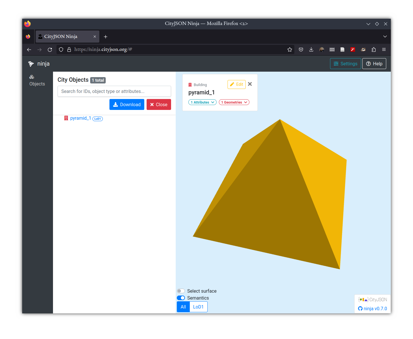
First, let's use a simple CityJSON viewer made available online, called "ninja," to view our pyramid. Head over to https://ninja.cityjson.org/ in a browser, and give it your pyramid.json file. You'll notice that ninja lists the pyramid with the "pyramid_1" name we gave it in the file, and if you click on it, a menu appears showing you attribute and geometry information, too.
Back in QGIS, we'll install a plugin that allows us to load CityJSON files. Under the "Plugins" menu, choose "Manage and Install Plugins." There search for CityJSON Loader, and install it.
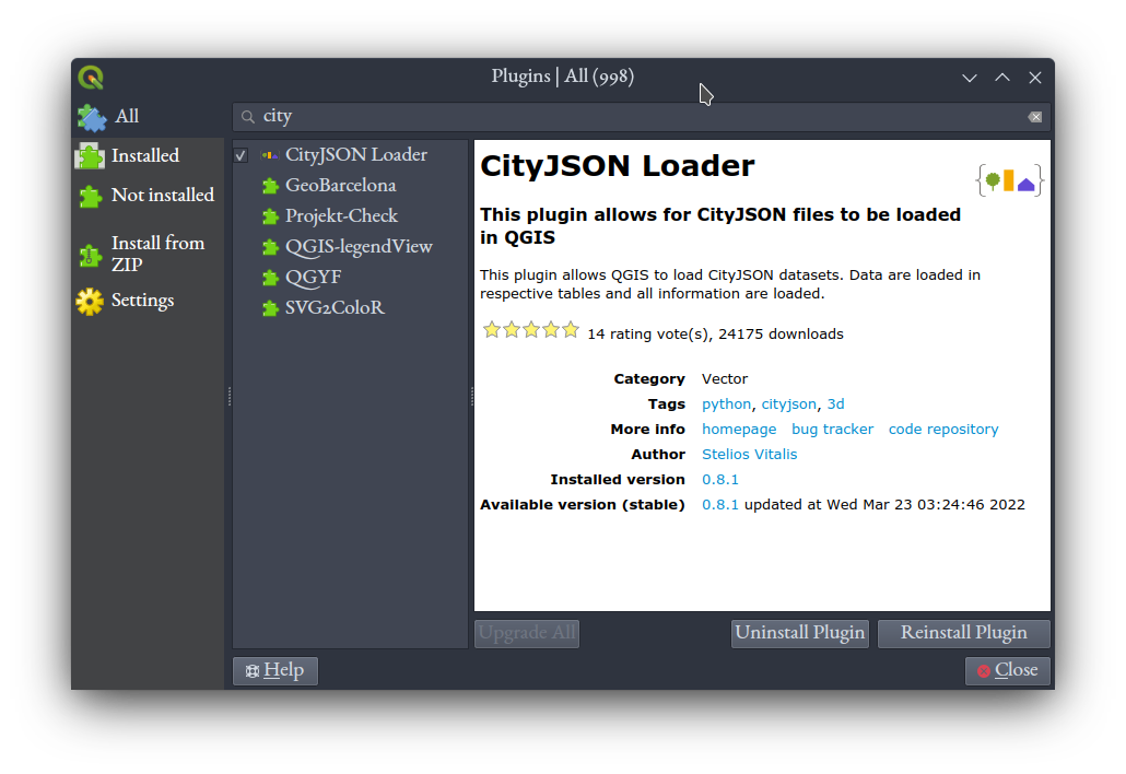
That will give you a toolbar in QGIS with a button on it, with an icon like this:  . Click that button, and load the pyramid.json file.
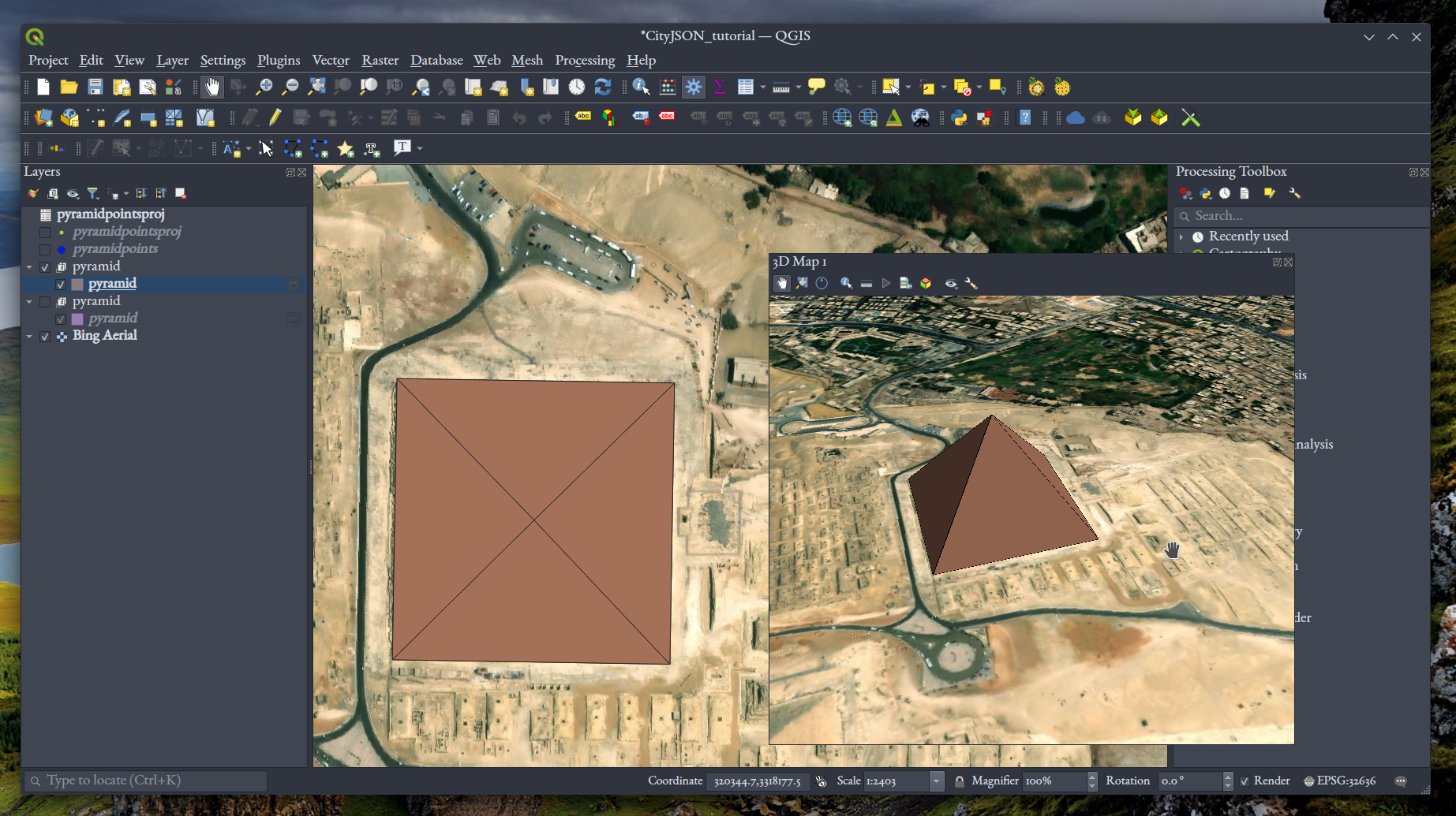
We'll get a 3D view here in QGIS. First, make sure the project file is in a projected coordinate system: use the same EPSG 32636 one we've used already under "Project," "Properties," "CRS." Then, with that set, open a 3D view under "View," "New 3D Map View." If you've got the Bing Aerial layer underneath your loaded CityJSON file, with a little moving around with your mouse (use the mouse wheel pressed down to orbit) you should see something like this:
Final notes on CityJSON
In the last code block above, we've got the whole file we set out to make, completed. Recall from the beginning of the tutorial that most practical CityJSON files are a lot longer than ours here: they contain multiple buildings (or bridges and trees, etc.) as CityObjects, rather than our single building. And buildings themselves can be much more complex, made up of separate, hierarchical parts with parent-child relationships, and features like windows, doors, and furniture. On top of that, files online are often stripped of spaces and new line characters to keep them small, so they don't readily lie on the page with the helpful indentations we've been using. Because of these things and more, CityJSON files will rarely be written from scratch like we did here, but rather will be generated by GIS and 3D software capable of reading, editing, and writing the files. So, a CityJSON file you encounter "out in the wild" will almost certainly be more complex than what we've done here (e.g., download one from https://3dbag.nl/en/viewer). But, this tutorial has, I hope, given you a solid (pun intended) understanding of the format in terms of geometry and attributes, and learning the rest of the format, along with a few software packages designed for reading, modifying, exporting and viewing it, should be easy with the thorough documentation available at https://www.cityjson.org/.
To whoever made the following meme, I am grateful.