Origin-Destination Mapping with Chicago Bikeshare Data
Paulo Raposo
pauloj.raposo@outlook.com
2022-10-02.
© Paulo Raposo, 2022. Free to share and use under Creative Commons Attribution 4.0 International license (CC BY 4.0).

Introduction
In this tutorial we'll use publicly-available Divvy Chicago bikeshare data to calculate and visualize trip durations and distances. We'll do some scripting to perform time calculations, some geoprocessing to calculate distances, and use kepler.gl, a free, online visualization platform to see our data.
Topics covered include:
- calculating time difference using a Python script,
- reprojecting and calculating distance from latitude and longitude coordinates,
- using kepler.gl to quickly visualize origin-destination trip sets.
Installing the software
We'll need Python 3 to do some calculations for us; install it if your machine doesn't already have it (if typing python --version into the command line gives you a version higher than 3.0, you're already set up). We'll also need QGIS 3 to do coordinate conversions and distance calculations. Finally, we'll need spreadsheet software, like LibreOffice Calc (free, as part of the LibreOffice suite at https://www.libreoffice.org/download/download-libreoffice/) or Microsoft Excel.
Getting the data
Let's go to Chicago!

Picture credit: Bhargava Marripati, from pexels.com.
We will visualize data from the city's Divvy bikeshare program. This bikeshare is station-based, i.e., bikes are rented from and returned to fixed locations throughout Chicago. Divvy makes historical usage data publicly available. Visit https://divvybikes.com/system-data and read about the nature of their data, to get a feeling for what they contain and what patterns they might be able to reveal. Importantly, too, read the Divvy Data License Agreement linked to on the website as well, to understand what conditions are placed on the usage of the data.
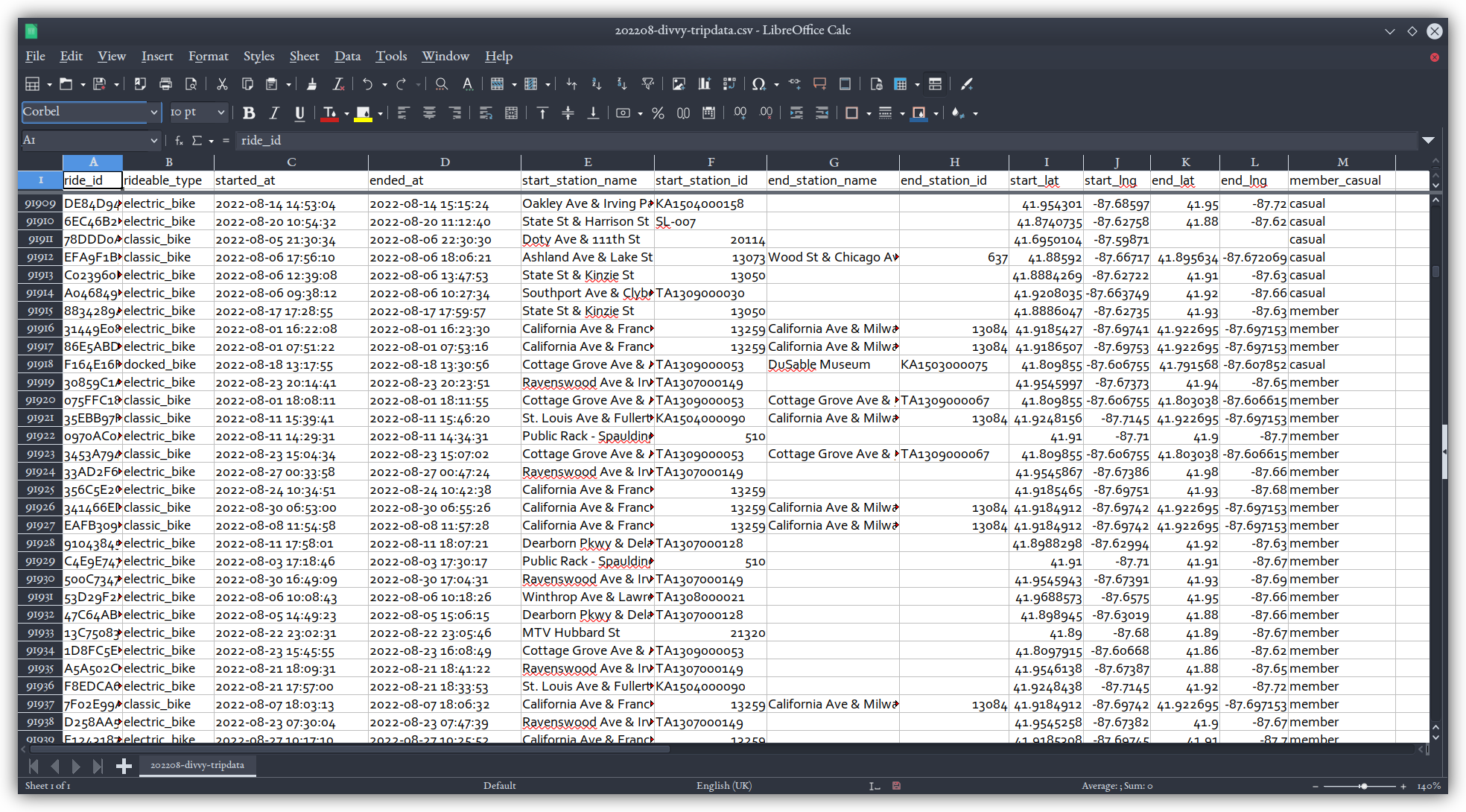
Follow the "Download Divvy trip history data" link on the webpage and select the file for August 2022 (the most recent at the time of writing this). Unzipping the file will give you 202208-divvy-tripdata.csv; if you get an empty __MACOSX folder as well, go ahead and delete that. The data is comma-delimited with double-qoutes around strings. You'll notice it has attribute fields for start and end dates and times down to the second as well as latitude and longitude of where those starts and ends were. There's also an attribute for the bike type, and sometimes there is station id and name information for the start, end, or both. Each row represents a trip taken by a rider.
Note that this file is somewhat large, so loading it in standard spreadsheet software, or in the kepler.gl environment we're about to do, may be a little slow --- be patient with your computer!
Calculating derived variables
The data set doesn't already contain trip duration information or trip distance, but we can calculate both of these for ourselves since there are latitude and longitude coordinates and start and end time stamps for each record.
Duration
We know, to the second, when each ride started and ended, because of the started_at and ended_at fields in the bikeshare data. So we can calculate the duration of each ride by subtracting the end time from the start time. That's striaght-forward logic, or course, but it gets a little tricker because of the multiple, nested units we track time by: seconds, minutes, hours, calendar dates, days of the week, etc. So we're going to make use of a Python package that handles all that time-keeping and calculating complexity for us, namely datetime.
Below is the source code for a script (also downloadable here). It will read our input CSV file, look for the start and end time values in the fields we tell it to look in, then do some fancy math to calculate those ride durations in seconds, outputing that in a new CSV field called seconds in a new CSV file, in the same folder as the input, but with _dur appended to the filename.
Don't worry if you don't understand the code, but do give it an honest try to, unless you're already comfortable with code like this. The lines with a
#symbol in front of them are normal language comments to help the reader understand what's going on in the instructions to the computer.
#!/usr/bin/env python3
# -*- coding: utf-8 -*-


#   .-.                              _____                                  __
#   /v\    L   I   N   U   X       / ____/__   ___   ___   ____ ___   ___  / /_  __  __
#  // \\                          / / __/ _ \/ __ \/ __ `/ ___/ __ `/ __ \/ __ \/ / / /
# /(   )\                        / /_/ /  __/ /_/ / /_/ / /  / /_/ / /_/ / / / / /_/ /
#  ^^-^^                         \____/\___/\____/\__, /_/   \__,_/ .___/_/ /_/\__, /
#                                                /____/          /_/          /____/


from datetime import datetime as dt
import argparse
import os
import csv


def main(in_CSV, start_field, end_field):

    # Define a new name for our output CSV by adding "_dur"
    # to the end, but not before the .csv extension. We
    # separate out the extension, then append it back in.
    in_path_no_ext, ext = os.path.splitext(in_CSV)
    new_path_no_ext = in_path_no_ext + "_dur"
    out_path = new_path_no_ext + ext

    # Open and read the CSV file.
    with open(in_CSV) as in_file:

        # Use A DictReader to read row by row.
        d_reader = csv.DictReader(
            in_file,
            delimiter=',',
            quotechar='"'
        )

        # Get the existing field names in the input file.
        field_names = d_reader.fieldnames

        # Add our new field to those.
        field_names.append("seconds")

        # Open the new, output CSV file.
        with open(out_path, 'w', newline='') as out_file:

            # Use a DictWriter to write new values to the output file.
            # Define its headers and write them, too.
            d_writer = csv.DictWriter(
                out_file,
                delimiter=',',
                quotechar='"',
                fieldnames=field_names
            )
            d_writer.writeheader()

            # Go through the input CSV row by row.
            for row in d_reader:

                # Convert the timestamps in the row to ISO format by replacing
                # the space with a capital T.
                start_ISO = row[start_field].replace(" ", "T")
                end_ISO = row[end_field].replace(" ", "T")

                # Save the timestamps as Python datetime objects.
                start_datetime = dt.fromisoformat(start_ISO)
                end_datetime = dt.fromisoformat(end_ISO)

                # Calculate the time difference by subtracting the end
                # datetime object from the start datetime object.
                time_delta = end_datetime - start_datetime

                # Get the time duration expressed in seconds using datetime's
                # total_seconds method.
                sec_count = time_delta.total_seconds()

                # Add this value to the set of values defined in `row`
                # as the value for the header "seconds".
                row["seconds"] = sec_count

                # Write the values defined in `row`, which now include our new
                # `seconds` value, to a row of the output CSV.
                d_writer.writerow(row)


if __name__ == '__main__':

    # Usage messages, and parse command line arguments.
    parser = argparse.ArgumentParser(
        description="A brief script to calculate trip duration in Divvy bikeshare CSV data."
    )
    parser.add_argument("INCSV",
        help="CSV file containing bikeshare trips."
    )
    parser.add_argument("STARTFIELD",
        help="Field in the input CSV with a time stamp for the beginning "
        "of the trip. Expecting `YYYY-MM-DD HH:MM:SS` format."
    )
    parser.add_argument("ENDFIELD",
        help="Field in the input CSV with a time stamp for the end "
        "of the trip. Expecting `YYYY-MM-DD HH:MM:SS` format."
    )

    args = parser.parse_args()

    main(
        args.INCSV,
        args.STARTFIELD,
        args.ENDFIELD
    )
python duration.py 202208-divvy-tripdata.csv started_at ended_at
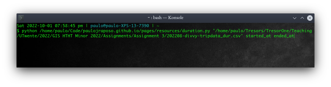
Below is what that looked like on my machine, with full paths to the Python script file and input CSV files. Note the single-quotes around the path to the CSV, because there are spaces in that path, which have to be put within quotes so that the terminal doesn't interepret them as the starts or ends of new arguments.
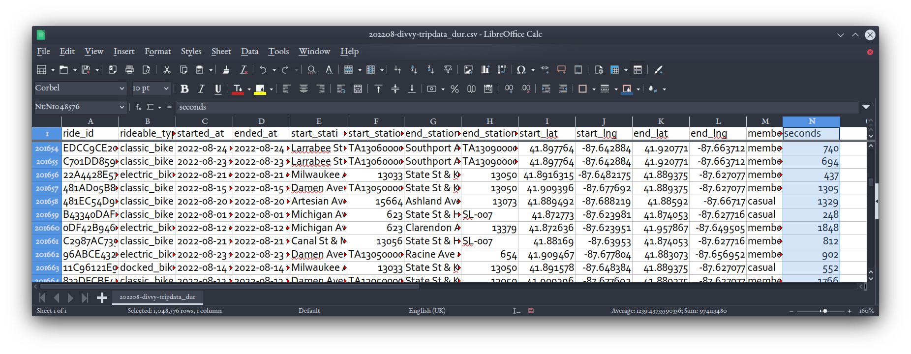
This command will take a few seconds, since it's a fairly big CSV. But then, if you open the 202208-divvy-tripdata_dur.csv file it produces, you'll see our new header with seconds written into it:
A nice little taste of the power of some Python!
Distance
We've got latitude and longitude coordinate pairs for the start and end points of every ride. We don't really know what route the rider took between those two points. But we can make some assumptions and evaluate them:
- We'll assume that most riders took a fairly direct route, not travelling more distance than they had to.
- Since Chicago has a very rectilinear street layout and any cyclist would be constrained by it, we'll calculate Manhattan distances, rather than direct Euclidean ones.
- We can compare travel distance to travel time: direct rides should have shorter travel times than meandering ones.
Calculating distances is going to be a little tricky, because the coordinates we have are latitude and longitude pairs, which are angular coordinates: one degree of longitude is, in most places on Earth, shorter than one degree of latitude, especially for a place as north on the globe as Chicago. So we can't treat those values the way we would two points on a Cartesian plane, with their distance being found by the Pythagorean theorem. We need to convert the coordinates first. Fortunately, a GIS is just the tool to do that for us.
Note: It's possible to calculate distances between lat,lon pairs using the Haversine formula. But instead of coding that math, we'll use the abilities already standard in QGIS (and just about any competent GIS, too).
A good coordinate system to use is the Universal Transverse Mercator, because distance measurements within one of the 60 zones around the world can be made with very good accuracy in all directions. Chicago falls neatly into Zone 16 North.
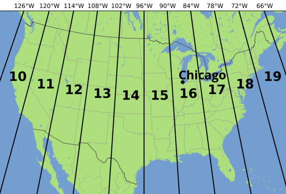
Adapted from image by Chrismurf at https://commons.wikimedia.org/wiki/File:Utm-zones-USA.svg.
Start up QGIS with a new project, then click the  Data Layers icon (or press Ctrl + L) to get the dialog that allows us to load data. Choose the "Delimited Text" tab, and select your
 202208-divvy-tripdata_dur.csv file. Set the X field to start_lng and Y field to start_lat, and leave the Geometry CRS at the default, WGS 84.
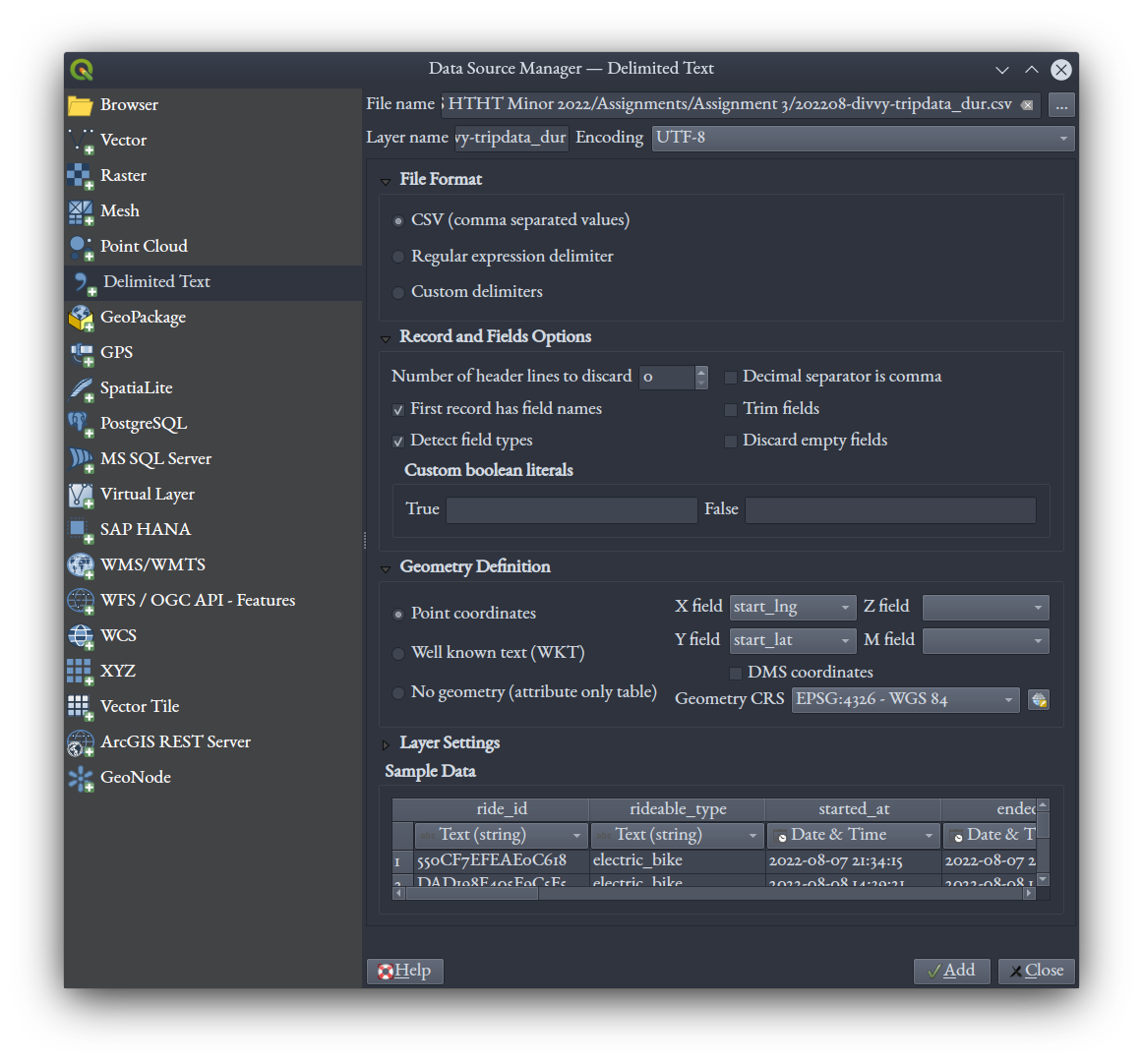
Click "Add." It might take a few seconds to load, as it is a fairly big text file.
Right-click the layer and choose "Export," "Save Features As." Use the GeoPackage format. Call it bike_starts.gpkg. Importantly, click the ![]() icon to get the CRS definition dialog. In the window that comes up, search for 32616, which will bring up the "EPSG:32616 - WGS 84 / UTM zone 16N" coordinate system option --- choose that one.
icon to get the CRS definition dialog. In the window that comes up, search for 32616, which will bring up the "EPSG:32616 - WGS 84 / UTM zone 16N" coordinate system option --- choose that one.
![]()
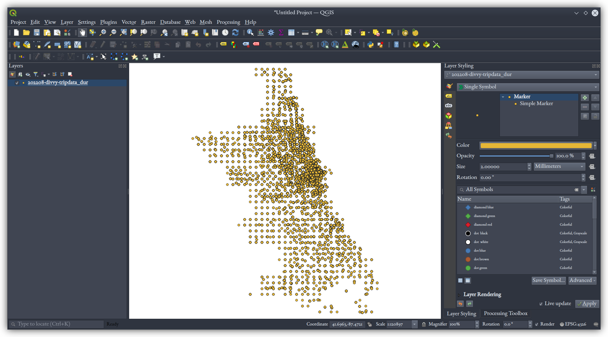
Upon clicking "OK," QGIS will convert the coordinates of each point into the UTM zone we asked for, and produce a GeoPackage file where those are the coordinates used to store the points. In the main QGIS window, you'll see the points from the two layers, your CSV and this new GeoPackage, are directly on top of each other --- they're in the same places, but now defined using different coordinate systems, and the GeoPackage coordinates are ones we can use to easily calculate distance with. At this point, remove the CSV layer from your QGIS project.
We need those Cartesian UTM coordinates explicit in the attribute table so we can mathematically manipulate them later. Right-click the GeoPackage layer and open the attribute table for it, including our seconds field (again, this opening might be a little slow). You'll see exactly the same table we saw before with spreadsheet software. Click on the "Open Field Calculator" icon (or press Ctrl + I).
![]()
Once in Field Calculator, leave the default "Create a new field" checked, call it start_eastings and set it to "Decimal number (real)" type. In the expression window, type $x to get the x-axis coordinate, which is given in "eastings," or meters eastward from a reference origin point, in the UTM coordinate system.
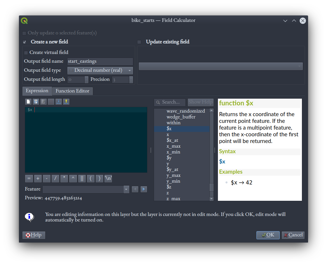
Click "OK" and the let the computer work for a minute or two. When it's done, the Field Calculator will close, and you should see the new column in the attribute table populated with values.
![]()
Repeat the same Field Calculator process, but for a field named start_northings and the expression being $y.
The field calculations we've done are an example of an "edit" to a layer in QGIS; i.e., a change of the data source file itself. We started editing automatically upon running the Field Calculator. Once done calculations for both northings and eastings, right click the layer in the QGIS Layers table and choose "Save Layer Edits" (another operation that can take a minute or two), to save the new fields we've calculated to the GeoPackage file on disk. Right click it again and select "Toggle Editing" to stop editing the layer.
And then, repeat the process of loading the CSV into QGIS, but use end_lng for the X coordinate and end_lat for the Y. Save again to a GeoPackage file with the CRS defined at UTM Zone 16N, calling this one bike_ends.gpkg. And again, in the attribute table Field Calculator of that layer, calculate end_eastings with $x, and end_northings with $y. Save your edits and toggle editing off.
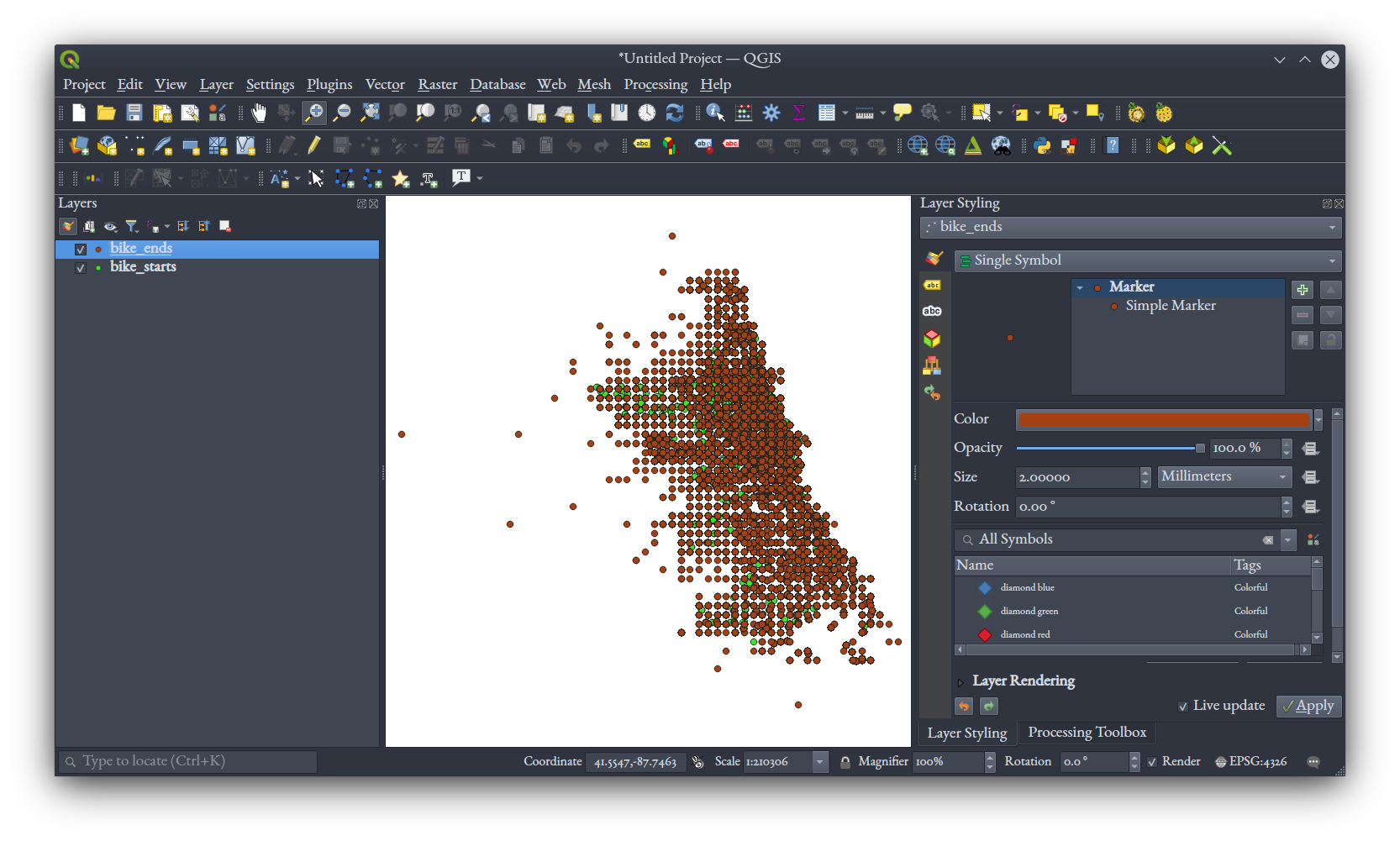
It would be nice to have these two coordinates, for starts and ends, in the same table, so let's perform a table join in QGIS to achieve that. You should have two layers in your QGIS project now, one for starts, another for ends:
Remember that the original bikeshare data had a field called ride_id, with a unique identifier for each of the 785,932 rides in the data. That field exists in both our bike_starts.gpkg and bike_ends.gpkg files, and we'll use it to perform a table join. In the main QGIS window, right click your bike_starts layer and select "Properties," then selecting the "Joins" tab. Click the + symbol near the bottom to define a new join, setting the "Join layer" to bike_ends, and both the "Join field" and "Target field" to ride_id. Tick the "Joined fields" option, and in the list of fields below it, tick the boxes for both end_eastings and end_northings. Selecting "Custom field name prefix," erase the text there so it's blank.
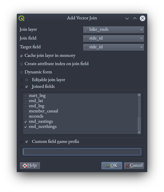
Click "OK" in this dialog, and "OK" again in the Properties dialog, and return to the main QGIS window. Opening the attribute table of bike_starts now you'll see the two fields from bike_ends that we chose in the join now appended to the table. Had we not selected a custom field name prefix they would have had bike_ends_ prepended to their names.
![]()
Save your QGIS project file --- that join is defined there.
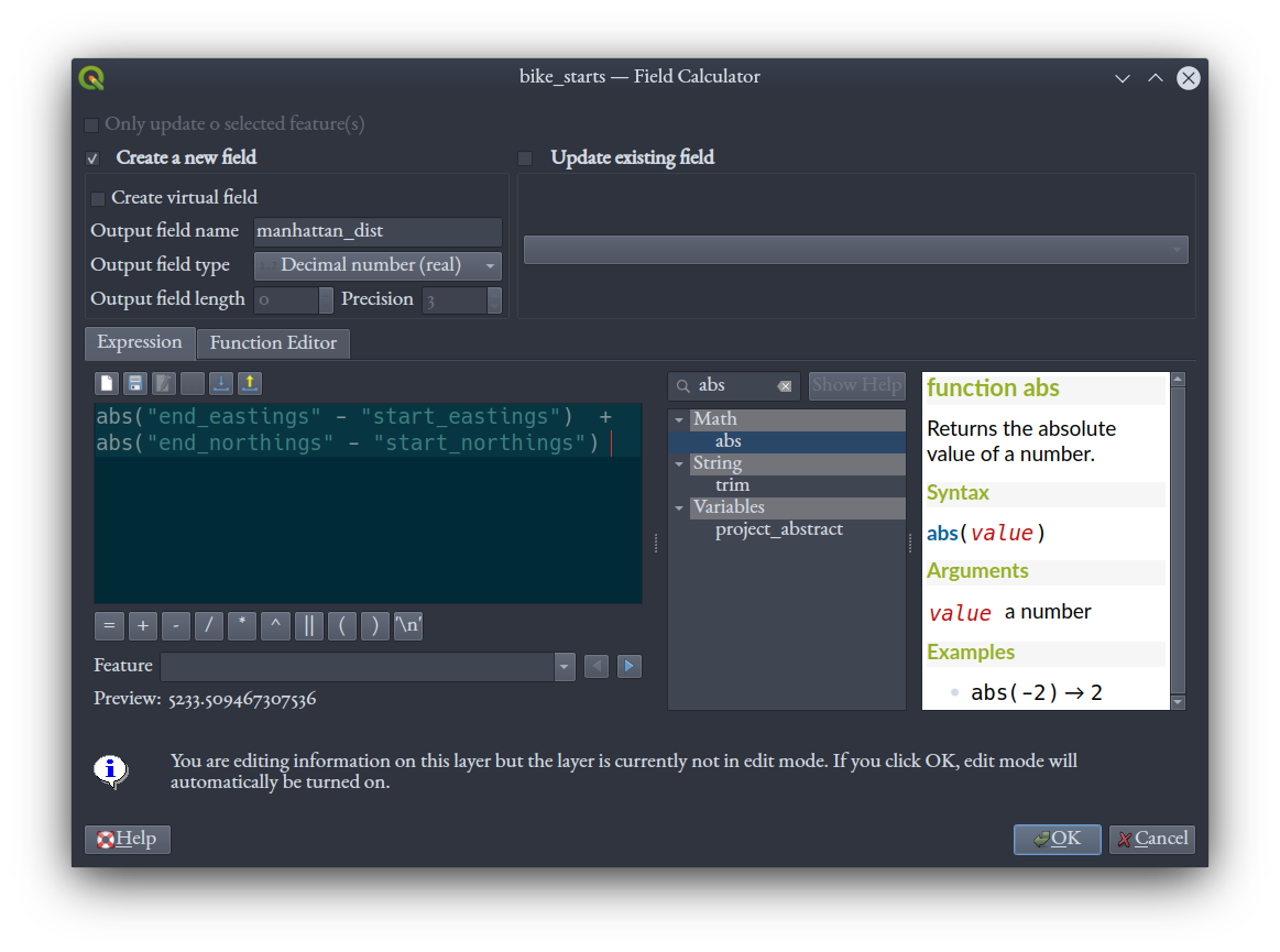
We're finally ready to calculate Manhattan distance! Again in the attribute table of bike_starts, open the Field Calculator, and calculate the Manhattan distance of each trip into a new, "Decimal number (real)" field using this expression:
abs("end_eastings" - "start_eastings") + abs("end_northings" - "start_northings")
Once it's done, remember to save edits and toggle off editing of the layer.
The Manhattan distance reveals some interesting issues with this data! Some rides get a distance of zero, though they have non-zero duration. Here's two examples highlighted, and we can see that for each, the start and end spatial coordinates, both in latitude and longitude pairs and in eastings and northings, are indeed the same.
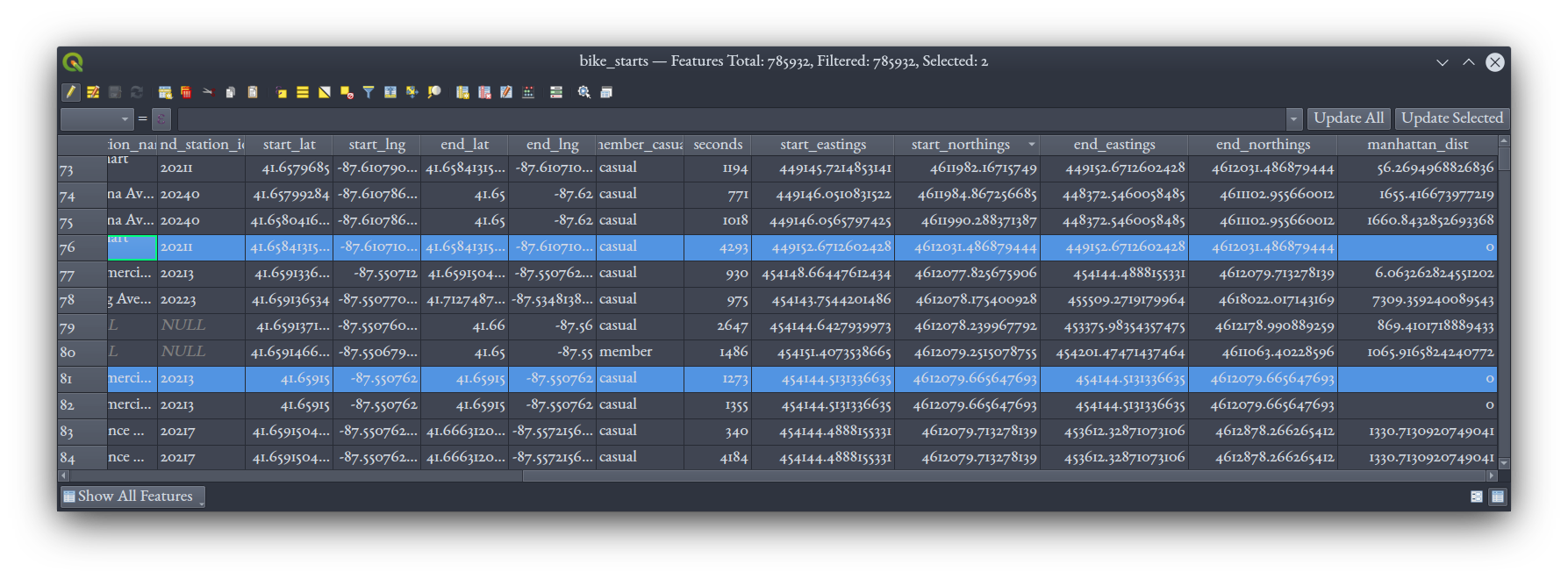
This makes sense: some riders took a bike and returned it to the same docking station.
Note: We've got eastings and northings, and Manhattan distances, to a ridiculous number of deminal places, given that the units are meters. The computer calculates to the precision it was asked to, and it doesn't ask questions about why you need to know where a bike ride started down to the nanometer. It's actually pretty common to find such spurious precision in GIS. If this were important, we should consider rounding these values off to something more realistic; for our purposes here, we'll leave the numbers as they are.
Visualizing rides
We've computed the distance and time data we're interested in. Let's use https://kepler.gl/, a free, online visualization tool to get some visualizations of these data. We'll export back out to CSV for that.
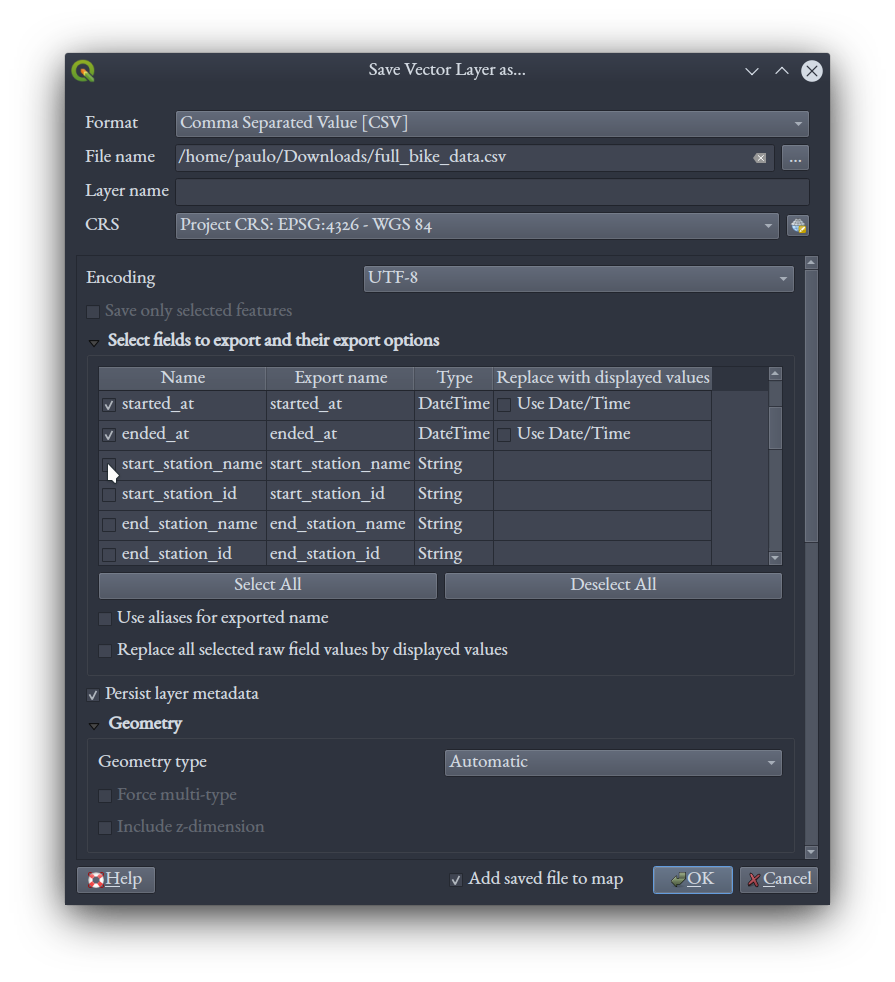
In QGIS, right click the bike_starts layer and export it. Choose CSV as the format, name the file full_bike_data.csv, and set the CRS to WGS 84 by searching for 4326, the EPSG code for WGS 84. To decrease the size of the output file, let's deselect some attribute fields we don't need, namely start_station_name, start_station_id, end_station_name, and end_station_id. Keep the rest at default and click "OK."
You can save your QGIS project and close QGIS at this point.
Open up your full_bike_data.csv file in spreadsheet software and confirm you've got seconds and manhattan_dist fields.
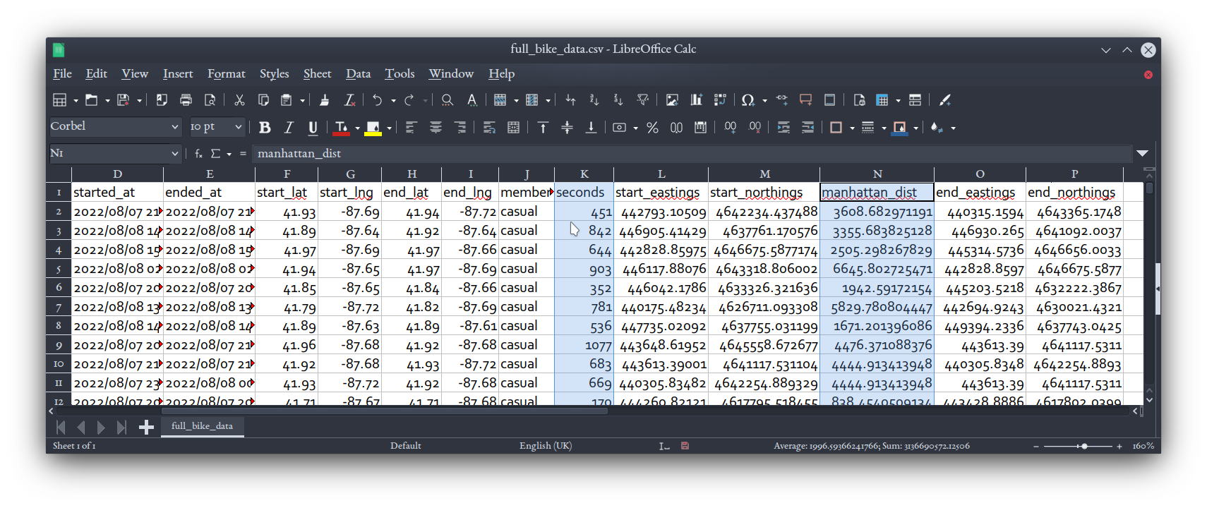
By now we've done several million calculations to get all theses data points for our approximately 700,000 rides. Be nice to your computer. ☺
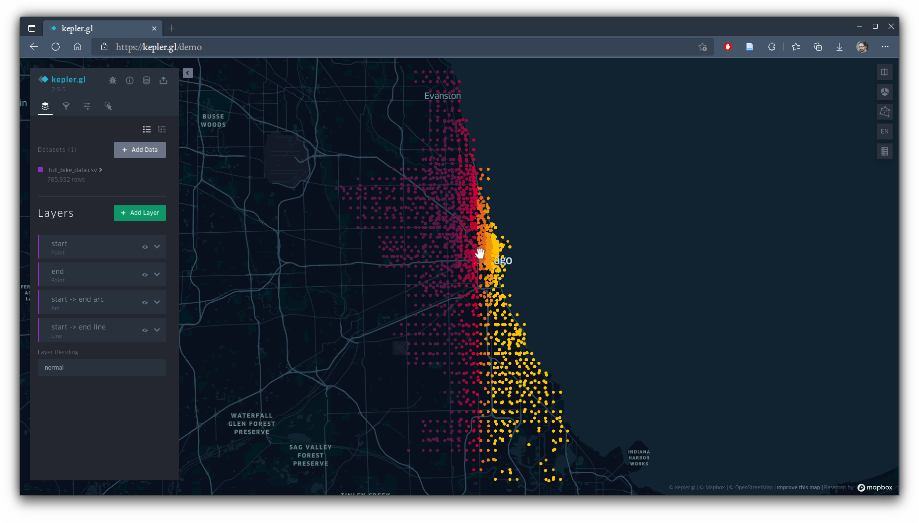
We'll visualize these data in 3D prism maps using kepler.gl. Visit https://kepler.gl/ with a Chrome-based browser (better interface rendering with this webapp) and click the "Get Started" button to load the demo webapp. You can then immediately drag-and-drop the full_bike_data.csv file into the app (or select it via browsing), and after reading through it, kepler.gl will make some guesses about the kind of data you just gave it (i.e., which field means what and how to deal with the points in the dataset) and how it can be symbolized. The interface is fairly straight-forward, but experiment with all the options available on the menu to the left, some of which are behind small and subtle buttons: you can add or remove layers, toggle their visibility, change the CSV fields they're driven by, change whether they're hexagon-based or square-based bin maps, among other things.
Kepler has determined that it can map start points, end points, and 3D arcs or flat lines between points, all on it's own. Let's tweak and add things now. Toggle off all the layers except the arcs (click the eye icons for them), and switch to a 3D view (using the cube button in the upper right). Click the downward chevron on the arc layer to open more options. Click the 3 dots beside "Color" and, in the "Color Based On" dropdown menu, select our seconds field. Lower the opacity to around 10%, and set the stroke to 1 pt. You should get something like this:
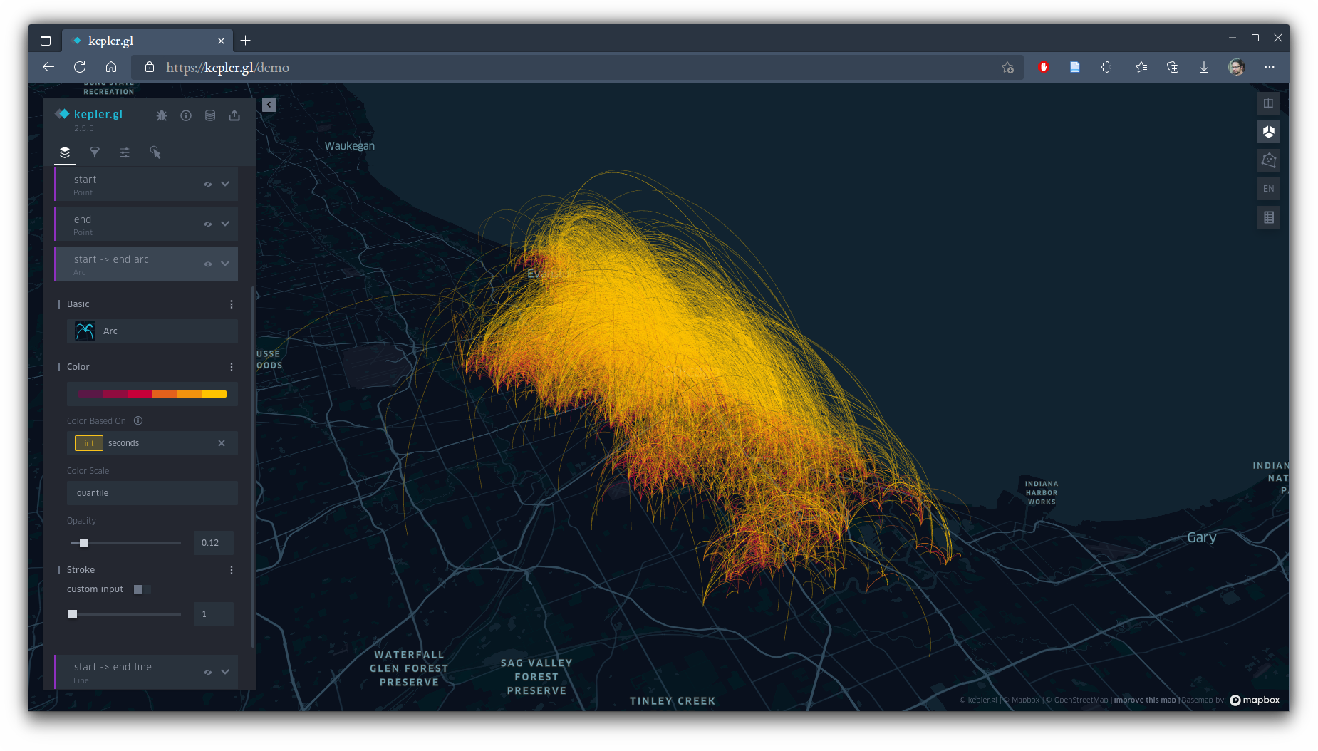
This is cool, but it's also a hot mess in terms of being analytically useful. We can interactively clean it up by adding a filter. In the "Filters" tab (the little funnel icon), add a filter on the manhattan_dist field.
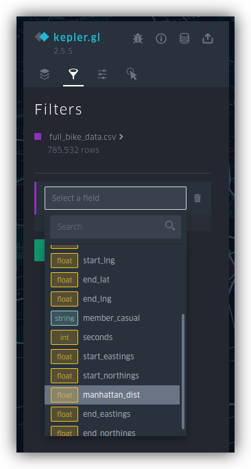
You'll get a histogram you can slide on for upper and lower bounds.
Under the "Interactions" tab, remove the fields in the Tooltip list, and add manhattan_dist and seconds, so that's what you're shown when you hover over an arc.
![]()
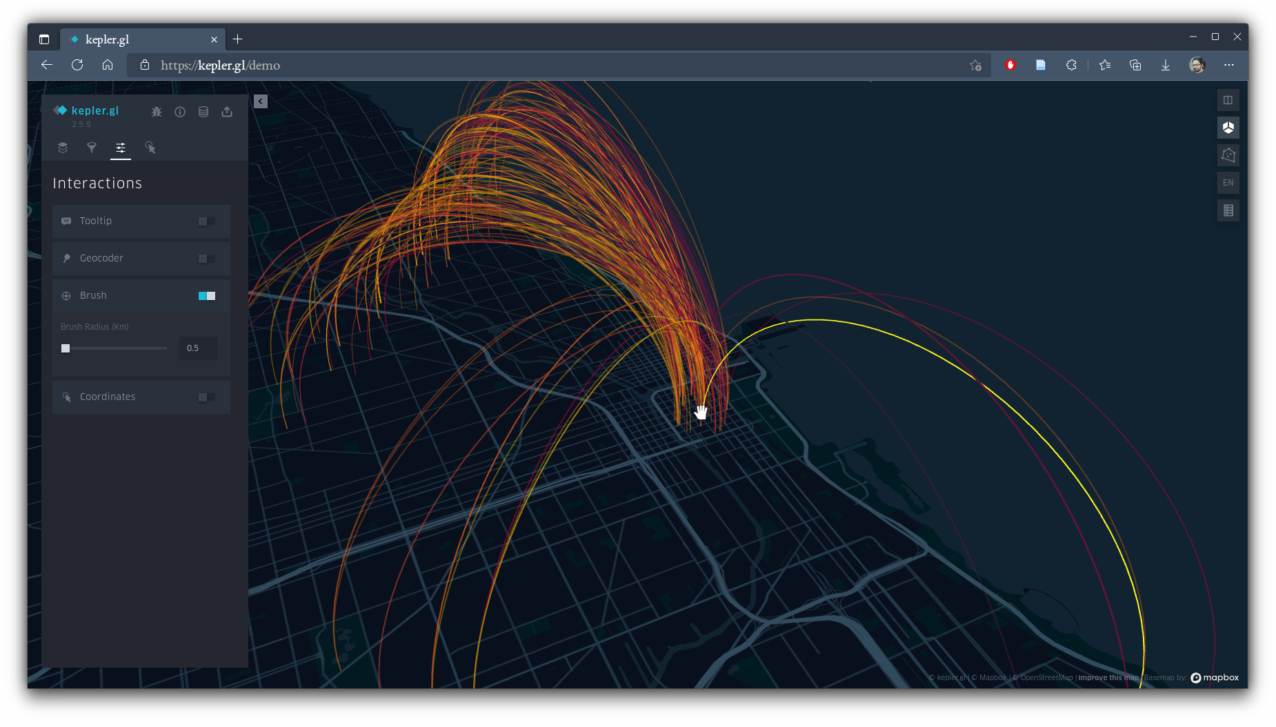
Also try the "Brush" interaction method, moving your mouse cursor over map slowly, showing you only those paths that extend from that point.
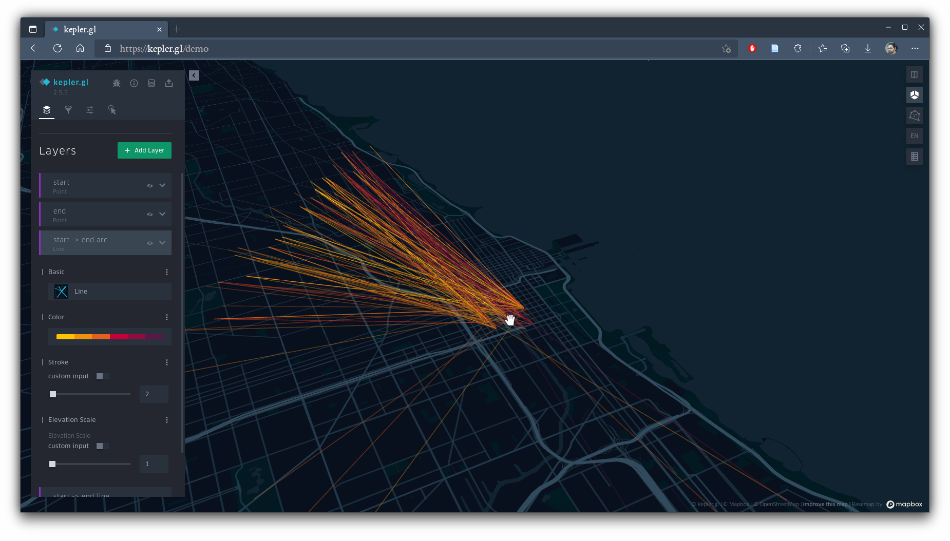
On the layers tab, under "Basic" for this layer, change the type of map to "Line." Still using the brush interaction, you should get a faster and clearer representation --- a nice example of how flashier is not always better! You might notice, as I did, that as you move around the downtown core (see my cursor location below), most of the other ends of the lines are north of it, and the few that are south seem to be further away... a clear pattern among the bikeshare users.
Now let's toggle off the line map, and toggle on the layer for ride starts. To make a 3D prism map, use the "Grid" map type with "Height" activated. Adjust "Radius" and "Elevation Scale" as you see fit so that bin size and vertical height make for visible patterns. Scroll down and open the "Height" options with it's 3-dot icon, and set "Height based on" to seconds, and "Aggregate Seconds by" to stdev (standard deviation).
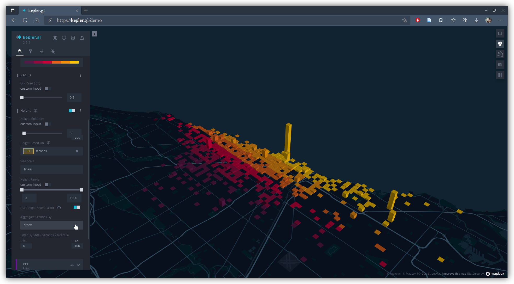
Change the aggregation type, and see how radically the map can change.
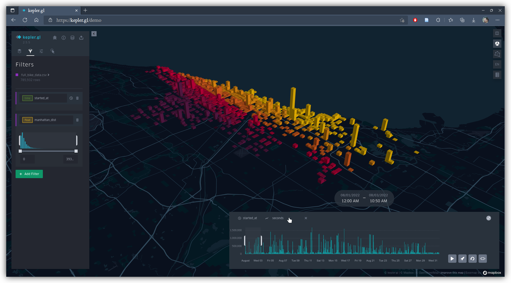
To add a temporal dimension, use the "Filter" tab again, and add a filter based on started_at. Kepler recognizes this field as a date and time, and will give you a time line at the bottom of the screen. On that timeline, click "y axis" and select seconds. You'll have options to narrow the snapshot sample window using two sliders, and the ability to play the data back in video time series, and if you've still got the manhattan_dist filter on, you can slide to select on that histogram too, something like this:
Conclusion
Spend some time tweaking and experimenting with the symbolization of your data layers among the options kepler.gl makes available. See if you can gather insights about days of the week that riders are most active, or parts of the city that tend to be more or less connected to each other by rides. Make use of more and multiple simultaneous filters to narrow down subgroups of riders, and consider things like aggregation method carefully. Reflect on what the strengths and weaknesses of visualizing these data this way are.
And have fun.