PDAL Tutorial - Basic LiDAR Data Handling and DTM Creation
Paulo Raposo
pauloj.raposo@outlook.com
2021-02-15, revised 2021-03-01, 2022-09-11, 2023-09-12, 2024-09-18, 2025-09-20.
© Paulo Raposo, 2021. Free to share and use under Creative Commons Attribution 4.0 International license (CC BY 4.0).

Introduction
In this tutorial, we'll use publicly-available LiDAR data and the open source and free software packages PDAL and QGIS to create a high resolution digital terrain model (DTM) that we can use in maps and 3D visualizations.
Installing the software
We'll need three free, open source packages for this tutorial: Anaconda, the Point Data Abstraction Library (PDAL), and QGIS 3. All three work on any of Windows, Mac or Linux operating systems. If you haven't already got these, please follow the appropriate instructions each package team provides (they're rather easy to install, and free):
- It's easiest to get PDAL through the Python distribution, Anaconda. So, please first install Anaconda.
- Then use these instructions to get PDAL via Anaconda: PDAL Quickstart.
- Finally, for further processing and visualizing our results, install QGIS 3.
Now let's see our study site and gather data for it.
Mount Saint Peter
Not all of The Netherlands is flat!
Let's look at a plateau in Maastricht, at the southern tip of the country, called Mount Saint Peter, or "Sint-Pietersberg" in Dutch. The site has been a rock quarry for hundreds of years, until operations by the most recent quarrying organization, ENCI, stopped there in 2018.
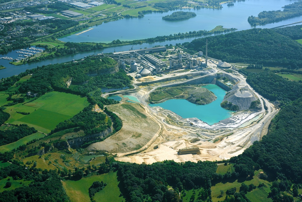
Above, the ENCI quarry site (photo credit: publicspace.org).
The site has been reclaimed and redesigned as a public park open to visitors. Follow these links to learn about the history of Mount Saint Peter and the quarry operations (look for the option to change to English as necessary):
- https://en.wikipedia.org/wiki/MountSaintPeter
- https://www.publicspace.org/works/-/project/k219-enci-quarry-reclamation-and-public-landscape-park
- https://www.rademacherdevries.com/luikerweg/
Being a plateau with artificially-altered morphology, the site offers an interesting study in 3D space and time analysis and visualization. Let's get some LiDAR data for the site.
The Actueel Hoogtebestand Nederland (AHN) is a Dutch series of datasets recording elevation throughout the country. There are presently several iterations through time of the AHN that are publicly available online. Each dataset is published with raster elevation data and the LiDAR point clouds from which it was generated. The datasets give us snapshots in time, because they were made in temporal succession:
- AHN 1: 1997-2004
- AHN 2: 2007-2012
- AHN 3: 2014-2019
- AHN 4: 2020-2022
- AHN 5: 2022-2024
Note: Since this tutorial was first written, AHN 4 and 5 have been released, and AHN 1 seems to have been taken offline.
Skim through this AHN presentation to gather some basic knowledge about the dataset you'll be working with.
We'll use the source LiDAR point cloud and make our own elevation raster. Visit the following link, where a map makes it easy to download all the currently-available AHN datasets on a tile by tile basis. Be sure to have the "Kaartbladen met downloadlinks" option selected in the settings menu at top left.
https://apps.arcgisonline.nl/hoogteviewer/
Pan and zoom to the tile that covers our area of interest in Maastricht (on the southern edge of the country) and click on it. In a pop-up you'll see links for several downloads across the AHN products. We'll use AHN 3 (you could always repeat the steps below for the other datasets and compare the change to the site over time). Select the AHN3 puntenwolk ("point cloud") dataset indicated in the following image:
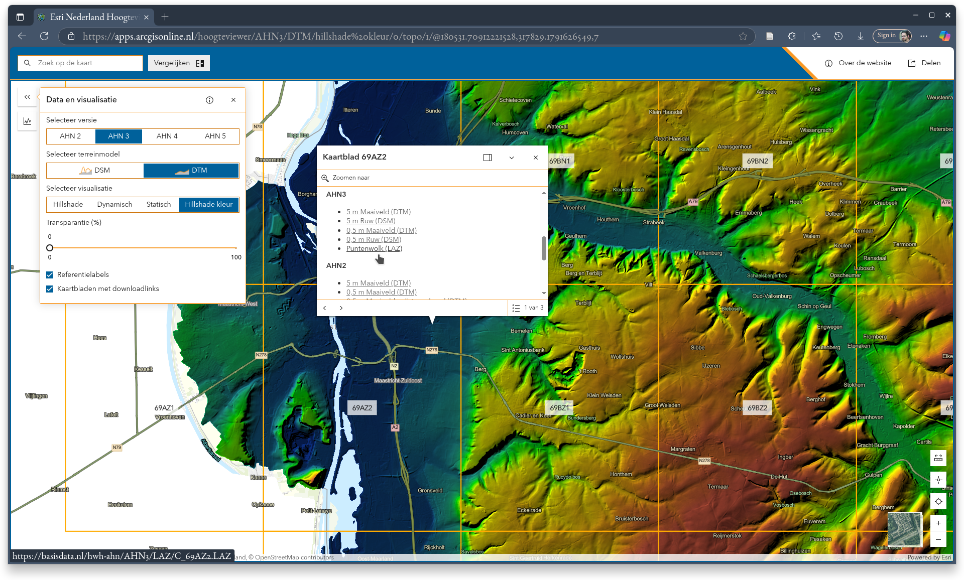
Important: These are fairly large files! The AHN3 one is 2.3 GB. LiDAR point clouds typically are large files containing millions of points. It may take a few minutes to download them. Some come as .zip files that you'll have to decompress to .laz files, which are themselves a compressed version of .las files (but there's no need to decompress .laz files before working with them). Running processing routines over them can take a while too, so expect to set things running and have to wait a few minutes or more for the results.
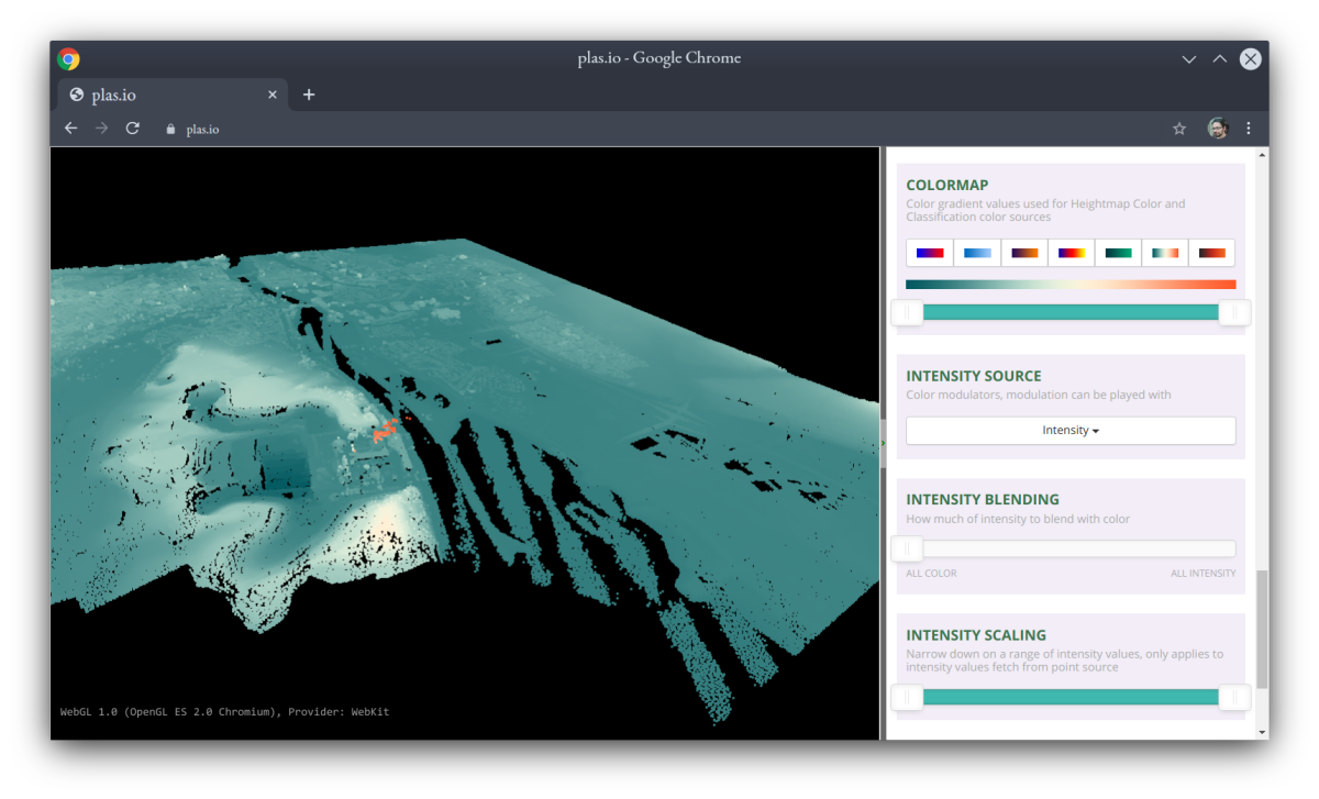
Let's have a look at this file to get a visual impression of the data. Visit the web app at https://plas.io/. On the right toolbar, set the "DENSITY" setting to the lowest (for the sake of speed, this will only render 10% of the points), and above it in the "FILE" section, browse for your LAZ file. Once it loads, and when you fiddle with colour options lower down in the panel, you should have an interactive view something like this:
LAS and LAZ files
It's important to know a little about LAS and LAZ files, the formats geospatial LiDAR data often come in. LAS is an open standard for point cloud data files, established by the American Society for Photogrammetry and Remote Sensing (ASPRS). LAZ is simply a compressed form of LAS, itself also an open standard.
For our introductory discussion here, all that's important to know is that LAS and LAZ files, from versions 1.1 to 1.4, have a standardized classification assigned to each point, reflecting where on the landscape that point is believed to be (e.g., on the ground, on a tree-top, etc.). Typically, when you download a point cloud from a data provider, they will have processed the bare data and assigned codes to each point already (though this is not always the case, and these classifications can be made or remade if and when you want to). These classifications allow us to filter a LAS or LAZ file for points on the landscape objects we're interested in, like buildings or vegetation. A good, brief, introductory discussion on this is available from Esri here.
Detailed information on this format in its latest version (1.4) is available here.
In this tutorial, we're interested in bare ground, and in the standard LAS classification, that's class 2.
Let's compute!
Assuming you set up an Anaconda environment called pdalenv when you installed PDAL according to the instructions above (it was called myenv in their instructions), open a terminal (PowerShell in Windows, Terminal on Mac OS, or any of many options like Konsole or gnome-terminal on Linux) and activate that environment now:
conda activate pdalenv
You should then be able to invoke the PDAL executable that was installed along with the Python library, and get its help page, as seen below:
pdal -h
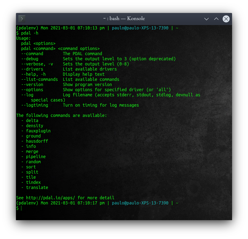
The "pipeline" command you see listed on that screen is what we want; it allows us to specify a multi-step operation to the PDAL program. Ours won't be many steps, but all the same. Pipelines in PDAL are defined as JSON objects, i.e., specifically formatted text with nested brackets. In this case, the JSON lays out a series of steps for PDAL to take. Below is the full JSON text we want (we'll break it down right afterward):
{
  "pipeline": [
    "/home/paulo/Downloads/LiDARData/C_69AZ2.LAZ",
    {
      "type": "filters.range",
      "limits": "Classification[2:2]"
    },
    {
      "filename": "/home/paulo/Downloads/LiDARData/dtm.tif",
      "gdaldriver": "GTiff",
      "output_type": "all",
      "resolution": "5.0",
      "type": "writers.gdal"
    }
  ]
}
Whatever OS you're using, use forward slashes (i.e.,
/) in your file paths in this JSON, even if you're on Windows (i.e., replace\with/). And to be safe, be fully case-sensitive in your paths, too. These are good practices, despite how they're not typically necessary on Windows.
The pipeline starts by defining the input .LAZ file. A comma comes before the next item. That item is a processing step. It's within curly brackets and has two statements, namely a declaration of a filter type (range), and a specification of which points to keep (classification 2, which are ground-classed points in LAS/LAZ files). The product of that processing step is fed to the next step, wherein five lines declare how we want to create a GeoTiff file at the path indicated, and at a resolution of 5.0 units (meters in this case, as the input file used meters in its coordinate system).
To use this pipeline, copy the whole text of it and save it in a text file; let's call it pipeline.json (or right-click and download this one I've already prepared). Note the two file paths: you'll need to edit those with a text editor (e.g., Notepad) to reflect where you saved the AHN LiDAR data on your system, and where you want PDAL to write the output DTM file.
Then, we run the program on the terminal with the following call, requesting a pipeline procedure and specifying the (path to) our pipeline.json text file:
pdal pipeline pipeline.json
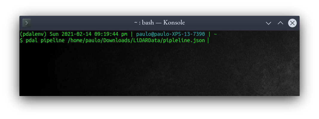
Friendly reminder: on the command line, if any file paths have spaces anywhere in them, be sure to enclose the whole path in double-quotes, because spaces mark the starts and ends of arguments to the terminal. So, if I had named the project folder differently than seen in the figure above, the full command might be like:
pdal pipeline "/home/paulo/Downloads/LiDAR Data/pipeline.json"
Press Enter. On my machine, with a fairly fast Intel i7 processor at 16 GB of RAM, this took just under 20 min to run—enough time to get a nice cup of coffee! As with most command line programs, there's no visual feedback about the program's progress until it's done and the command prompt returns, or until there's an error and a message for it is shown. If you want to, you could make sure things are running by looking at a process manager (e.g., Task Manager in Windows).
If you anticipate a command to PDAL to take a while and you want it to print status messages to the screen to reassure you it's working, add
-v 8to the end of the command. That asks PDAL to be very verbose (i.e., "talkative"). Or, you can just get used to the fact that in the terminal, it's normal to get no visual feedback while a process is still running as expected.
GIS processing and visualization
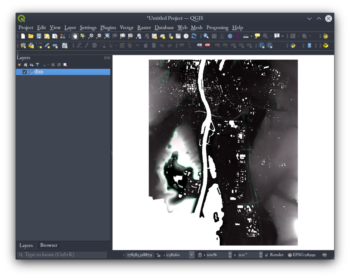
Fire up QGIS 3, and load the GeoTiff file we produced above. When it loads, QGIS will display a little icon  beside it in the Layers list to indicate it has no coordinate reference system (CRS). Click on that, and search for "28992" to find and select EPSG:28992 "Amersfoord / RD New," a virtually planimetric and equal-area projection for The Netherlands, and the one the original data came in. Set the project to that CRS too, under the "Project Properties" dialog. Then we'll be sure we're looking at the data using proper geometry.
What gets produced by PDAL above is a GeoTiff raster image, where there are grid cells defined wherever there were class 2 points in the input LAZ file. Elsewhere, there are blank, "nodata" cells (e.g., where there were building- or vegetation-classed points and no ground points, or no points at all). This raster has 6 bands; right-click it and select "Properties," and then under the "Information" tab you'll see that they represent the minimum, maximum, and mean elevation values of the points that fell into that pixel, as well as values for inverse distance weighting ("idw"), the point count, and the standard deviation in their elevation z-values.
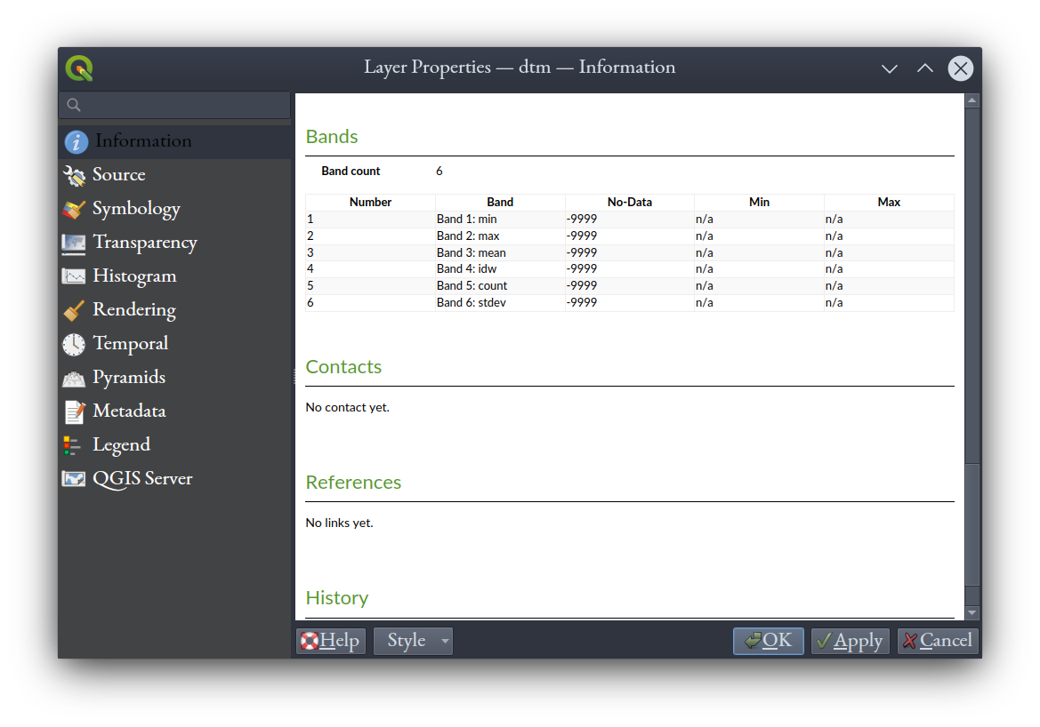
These statistics can be useful in advanced analysis of the precision of the surface you've created. For our purposes here, we'll just go with the mean elevation value in band 3. So our next step is to extract band 3 to its own file, a single-band DTM in its own GeoTiff.
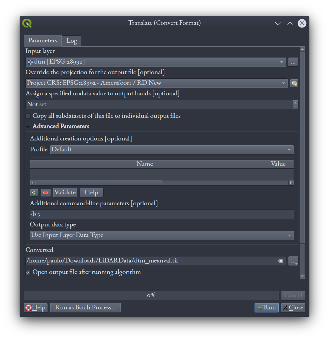
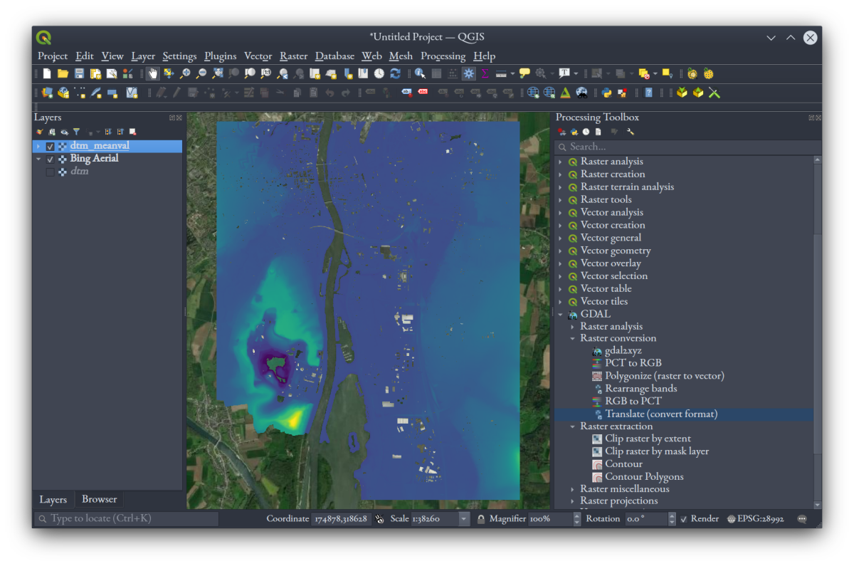
In the Processing Toolbox, go to "GDAL," "Raster Conversion," and select "Translate (convert format)." Make sure our raster is selected as the input with its EPSG:28992 coordinate reference showing. Under "Override the projection for the output file [optional]," select the project CRS, namely EPSG:28992 (this ensures the output will have the correct CRS identified as part of its file). Choose a location and name for the output GeoTiff raster under "Converted." Open the "Advanced Parameters" section, and under "Additional command-line parameters [optional]," write -b 3. This last bit asks GDAL to extract only band 3. See the full set of parameter choices below:
Click "Run." Your output will look very much the same as the layer before, but this one will have only one band, and will be recognized as an elevation raster because of this in the visualization tool we're going to use in a few steps. In the "Properties" window for this layer, let's go to "Symbology," and select "Singleband pseudocolor" as the "Render" type, pick a colour ramp, and press "Classify" and "OK."
To orient ourselves, we'll load a basemap using the XYZ data source feature in QGIS. Open the "Data Source Manager" by clicking on the  icon or pressing Ctrl + L. Under the "XYZ" tab, click new, and enter in the following name and URL data for Bing Aerial imagery:
Bing Aerial
http://ecn.t3.tiles.virtualearth.net/tiles/a{q}.jpeg?g=1
Click "OK," and with "Bing Aerial" selected in the XYZ data source window, click "Add" at the bottom of the screen. Accept the default options if QGIS asks you about projection transformation options for this layer. Close the "Data Source Manager" window to see the Bing imagery tiles loaded; these will update as you pan and zoom the map.
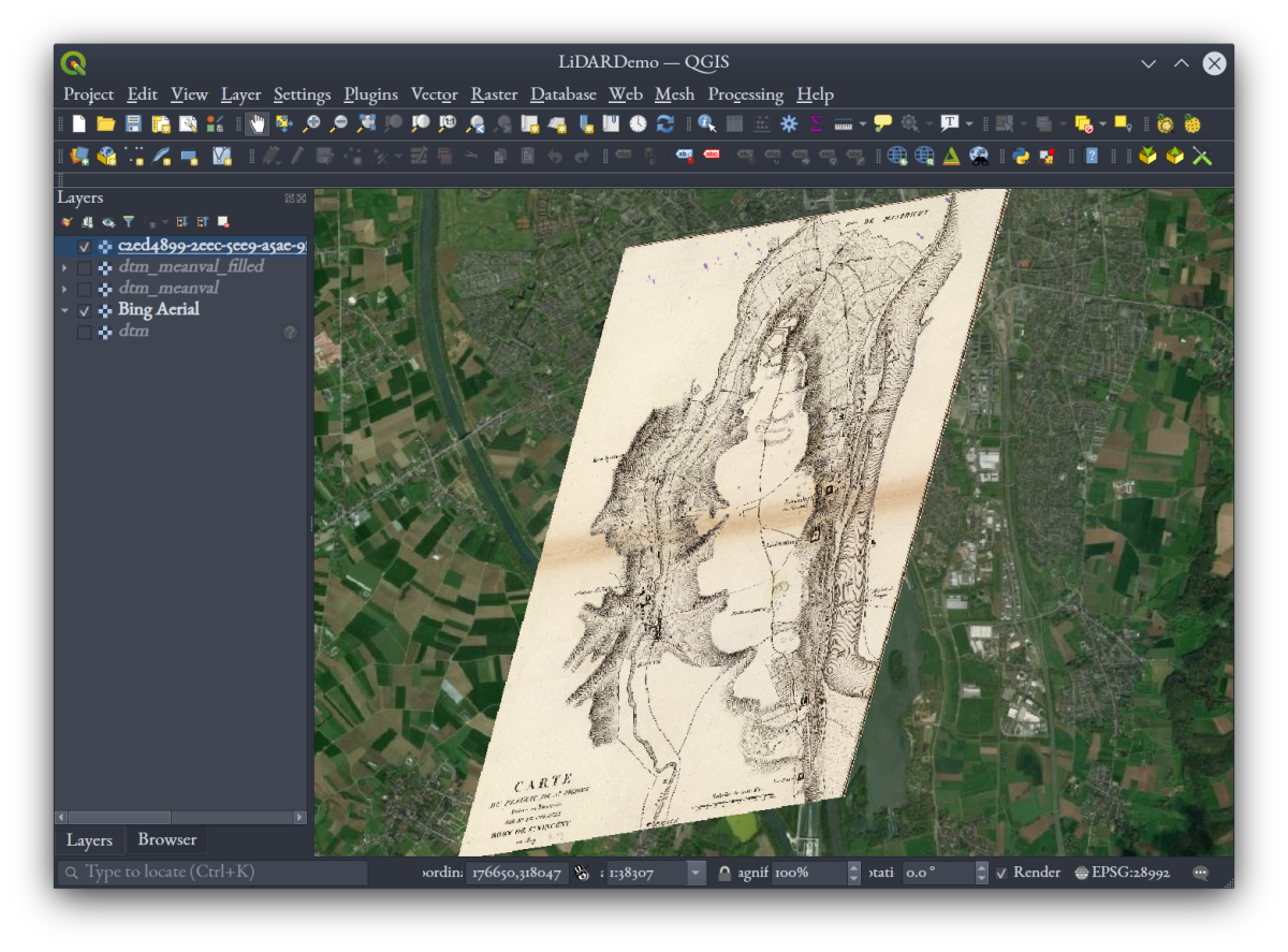
Once you arrange your layers so that the Bing imagery is on the bottom, your single-band DTM is on top, and the DTM from before is turned off, you should get something like this:
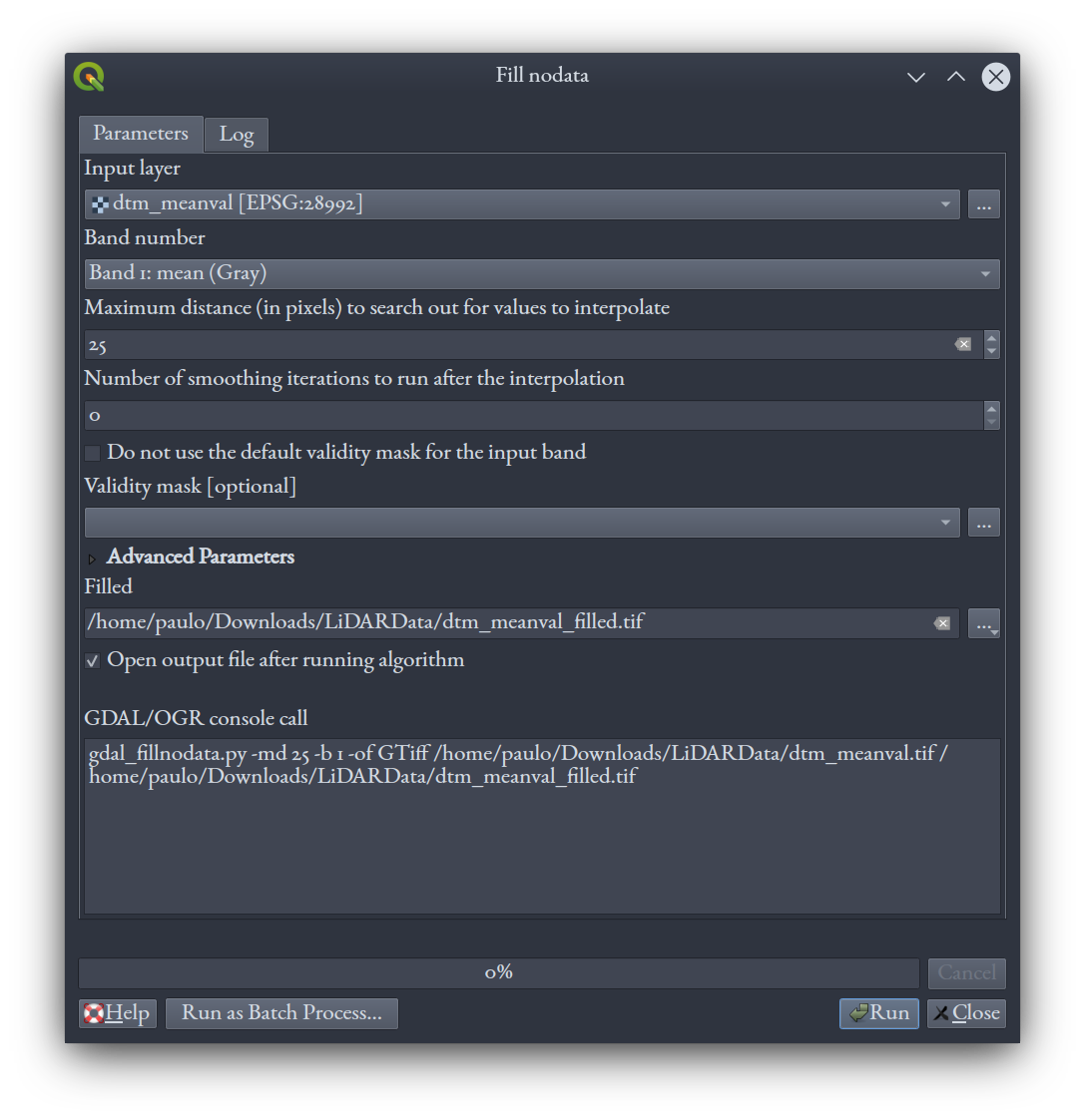
There are holes in the surface - wherever there weren't any ground-classed pixels for PDAL to work with when it gridded to 5 m. Some of these holes you'll recognize readily as buildings, and other are just empty spaces. To simulate unbroken ground, let's fill the nodata holes in our DTM by interpolating values for them from nearby pixels. In QGIS, under "Processing," find the GDAL tool "Fill nodata" under "Raster Analysis." Create a new GeoTiff file as output, having filled areas of nodata up to 25 cells:
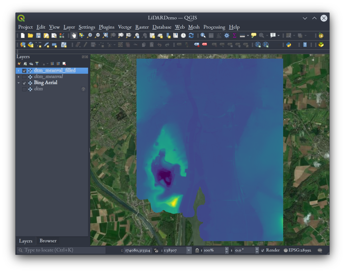
After applying a colour ramp the way we did before, your new layer should look something like this:
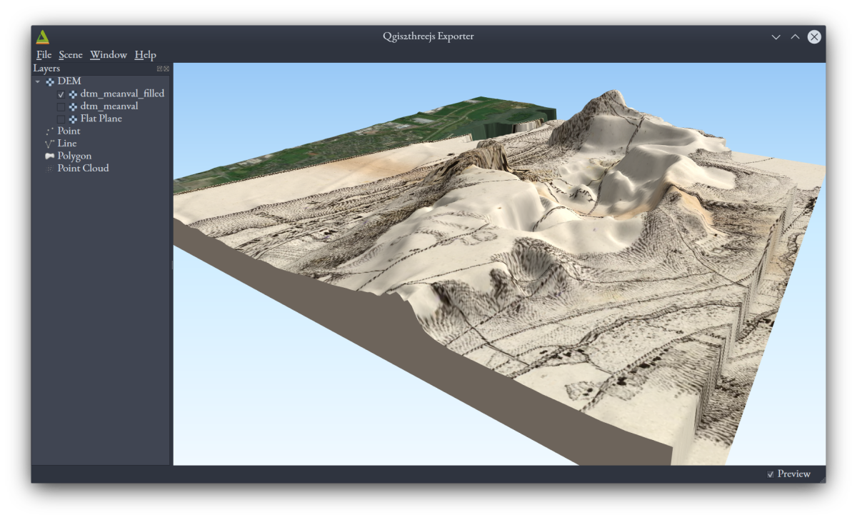
Let's see this in 3D! We'll use a plugin for QGIS called Qgis2threejs, to get an interactive, 3D visualization of our data. This plugin allows us to export a webpage from our QGIS project that gives the viewer the same 3D model we can see and manipulate. It also allows us to export the model to glTF format, which is useful in many different 3D software environments.
We need to install this plugin first (if you haven't already). In QGIS, go to "Plugins," then "Manage and Install Plugins." In the dialog that pops up, search for "qgis2threejs" and select and install it when it pops up. Then, under the "Web" menu, select the option for the "Qgis2threejs Exporter," or click on the icon  that may have appeared on your tool bar.
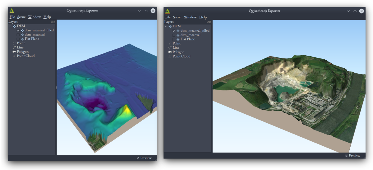
Follow this short Qgis2threejs tutorial for getting a 3D scene loaded with the plugin, but skip the parts about getting a DEM and setting its CRS, since we've already taken care of that. There's no need to export to glTF at this point either. Go to "Scene," then "Properties," and try setting the vertical exaggeration to 2 or 3. Toggling layers on and off in the main QGIS window will toggle them in this viewer, too, and panning and zooming there will change the extent rendered here. Once you've got your no-holes DTM set as the "DEM" in Qgis2threejs, you should be able to get views like these, when you zoom in on the main QGIS window and turn layers on and off:
Let's look at an interesting historical record of Mount Saint Peter! This 1827 map at the David Rumsey Map Collection illustrates the plateau and has been conveniently georeferenced for us. After making a free account with the site and logging in, you can use the "Export to GeoTiff" option near the bottom of the page and download the .tif file. Load it into your QGIS project. Notice how much has changed, with the plateau and the course of the Meuse river right beside it!
In Qgis2threejs, using the "Export to Web" option will produce a series of files and folders, all of which together make up a web page, if hosted on a web server. Note how in the tutorial an option is given for making a version of that webpage that can run locally (i.e., on your own machine without any web server technology). But even if you don't use that option and create a normal web page, you can view it from your local machine by setting up a basic Python web server in that directory.
Conclusion
The above tutorial has hopefully made you comfortable with the basics of handling LiDAR data to create layers you can use in cartographic and GIS contexts. Similar workflows with different tools are available in Esri's ArcPro software, and another powerful free and open source GIS, SAGA.
Notes on classified and unclassified LAS files
The above assumed that the LAS or LAZ files you're working with have classifications for each point, but sometimes that isn't the case. How can you tell? Using PDAL, of course.
On the command line, run the following on your file:
pdal info yourfile.las
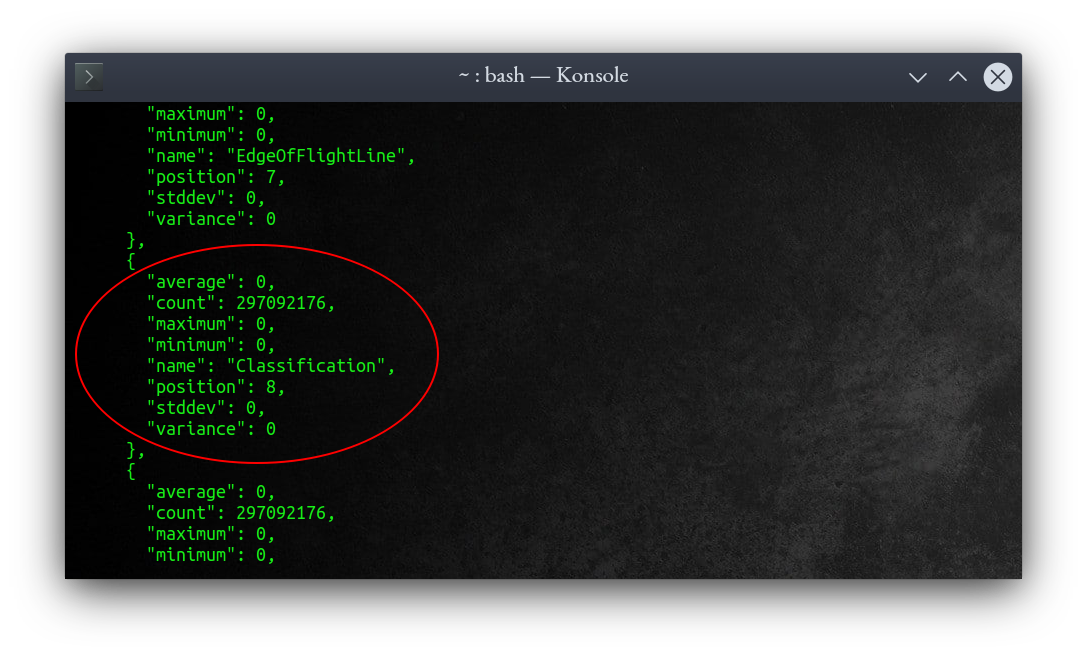
PDAL will read your file and print a JSON report of statistics calculated over the file and its attributes. It has to read the whole file, so it might take a little time (my laptop took about 6 minutes on a tile of AHN2 data). Once it prints, scroll through the output and look for the section on "Classification." Zero in the LAS file specification means that a point was never classified. If the minimum value for Classification is zero, you've got at least some unclassified points in this cloud (as was the case for AHN1 and AHN2 point clouds when I tried it, with all points unclassified):
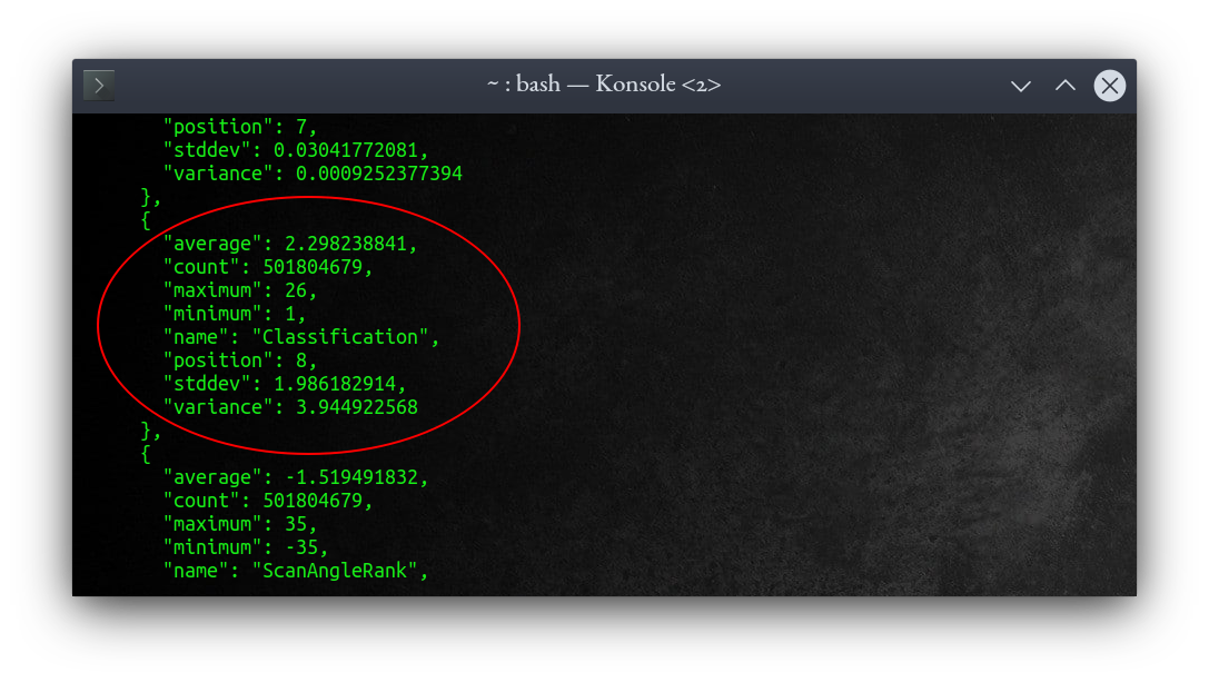
Conversely, if you've got values other than zero, you've got a classed point cloud (as was the case for AHN3 when I tried it):
If you've got an unclassified point cloud, no worries: you can use PDAL to classify points as ground, vegetation, etc., according to various algorithms PDAL comes prepared with. To get just ground points using default settings (class 1 "unclassified" points will remain too), use this command:
pdal ground -i myfile.laz -o myfile_ground.laz
Above, the -i flag simply indicates that the next thing is the (path to) the input file, while the -o flag indicates that the next thing is the (path to) the output file.
This is relatively computationally heavy! Don't do much else with your computer while this is running. On my machine, a tile of AHN2 LAZ data took about 30 minutes.
For our purposes here, this is good enough, but note that this is not fool-proof; the algorithms aren't perfect. There's more detail about how you can tune them for even more accurate output here.
What to do if you run out of memory
As mentioned above, running the ground classification PDAL tool is a relatively computationally heavy task. In desktop computing terms, the amount of RAM memory required is relatively high. Consequently, you might find that running the tool on a tile of AHN LiDAR might fail with an error message like "bad allocation," or "insufficient memory," and could happen some time (e.g., an hour) into the process. This depends on how much RAM your computer has available at the time of running the tool. My Ubuntu computer, for example, has 16 GB of RAM, and completed the task after using up all the available RAM, plus extra swap space. If your computer has a smaller amount of RAM, say 8 or 4 GB, calculating ground this way on a tile of AHN2 may overwhelm your system. But there are solutions to this problem!
1. Increase your virtual memory space
Virtual memory is persistent storage space (e.g., hard disk space), used as if it were working memory (i.e., random-access memory, RAM), typically when working memory is full. It is generally much slower to use virtual memory, but at least your programs don't crash. Different operating systems handle virtual memory differently:
- Linux systems (e.g., Ubuntu) use a "swap" space of a defined size.
- Windows 10 uses a "paging" file of a defined size.
- Mac OS X allocates virtual memory automatically, as necessary (unless you turn this feature off).
If you're running out of memory on either Windows or Linux, the first thing to do is to try increasing the amount of virtual memory allocated:
- On Windows, follow this tutorial to increase your paging file size.
- On Ubuntu 20.04, follow this tutorial to increase your swap size.
Then try running the PDAL ground tool again.
2. Tile your LiDAR data into smaller files
If adding more virtual memory doesn't work, you're simply trying to do more than your system can handle. So another solution is to break the work down into smaller pieces and do them in sequence.
PDAL offers lots of LiDAR handling tools, including one to partition a LAS dataset into smaller tiles. We'll use another pipeline to split our AHN LiDAR file up, with this pipeline JSON file:
{
  "pipeline": [
    "/home/paulo/Downloads/LiDARData/AHN2/g69az2.laz",
    {
      "type": "filters.splitter",
      "length": "2000"
    },
    {
      "type": "writers.las",
      "filename": "/home/paulo/Downloads/LiDARData/AHN2/tile_#.las"
    }
  ]
}
Above, we've defined a splitter filter that will make tiles as large as 2000 units (meters in our AHN LiDAR files) to a side. I chose tiles at 2000 m wide arbitrarily, because it would result in at least quartering the AHN tiles—feel free to try different sizes. There will be multiple output LAS files, and we write the output path with a # symbol, which will get replaced by 1, 2, 3, etc. As before, edit the file paths to reflect your own locations.
Then run:
pdal pipeline splittingpipeline.jsonAfterward, you run the ground classification tool described above on each of those tiles, in sequence.
And to finish, you merge however many smaller, ground-classified tiles back together with another pipeline:
{
  "pipeline": [
    "/home/paulo/Downloads/LiDARData/AHN2/ground_tile_1.las",
    "/home/paulo/Downloads/LiDARData/AHN2/ground_tile_2.las",
    "/home/paulo/Downloads/LiDARData/AHN2/ground_tile_3.las",
    "/home/paulo/Downloads/LiDARData/AHN2/ground_tile_4.las",
    {
      "type": "filters.merge"
    },
    "/home/paulo/Downloads/LiDARData/AHN2/ground_whole.las"
  ]
}
This tiling method likely introduces edge effects, where processing produces different results at the edge of the dataset than it would if the dataset weren't split up (i.e., if the various nodata areas corresponding to the outer limits of the dataset actually contained valid data). To mitigate those effects, the splitting tool can be used to make tiles that overlap each other by a defined distance, and a point-by-point comparison operation could be used when merging overlapping tiles back together—but for this tutorial, we'll skip the analysis involved in that.