Table Joining in QGIS 3
Paulo Raposo
pauloj.raposo@outlook.com
2023-08-13.
© Paulo Raposo, 2023. Free to share and use under Creative Commons Attribution 4.0 International license (CC BY 4.0).

 Image by Lance Grandahl, from Unsplash.
Very often in all sorts of data science and manipulation, including in geographical information systems (GIS), you have data stored across multiple tables that need to be associated with each other. This is often done by putting tables together, two at a time, with logic that matches certain rows from one table to certain rows from another. People in different specializations (e.g., dabases, GIS, data science) use different terms for this (sometimes because there are different details about exactly how the software does it), but merge and join are common. From here on, we'll call it a join (the more common term among people doing GIS).
Using simple example tables, we'll go through four different types of joins.
Table A contains records on five objects, each with a unique ID, and some colour and shape:
| ID | Colour | Shape |
|---|---|---|
| 001 | Red | Square |
| 002 | Orange | Circle |
| 003 | Blue | Triangle |
| 004 | Blue | Octagon |
| 005 | Yellow | Triangle |
Table B contains records of the same kind of objects, still with unique IDs, but this time with mass only, and the set of objects is different from those in Table A:
| ID | Mass |
|---|---|
| 001 | 12 |
| 002 | 432 |
| 005 | 3 |
| 006 | 4 |
So across these two tables, we have data for six different objects, each with a unique ID value. For five of those objects, we have colour and shape data, and for four of them we have mass data.
Keys
Across any two tables, corresponding rows might exist or not, and be in different sequences. We can't naively assume that rows will simply line up in order: there has to be a way of matching certain rows from one table to certain rows in the other. This is typically done using two special columns, one in each table, that contain values that match up identically across the tables. Those columns are called keys durring a table join. When in a database situation in which you are starting with a main table of data, and you're adding rows from another table (perhaps temporarily or "on-the-fly," meaning only while your program is running), those matching columns are called the primary key and foreign key, respectively.
4 Types of Joins: Left, Right, Outer, and Inner
In a lot of database terminology, the first of two tables to join is the "left" table and the second is the "right" one, same as they would appear if written out in any language that writes from left to right.
Left Joins
A left join means that all records from the left (or first) table will be kept, even if there's no corresponding matching data from the right (or second) table, and rows from the right table will be carried over to the join only if each has a match to some row in the left table. Here's the product of a left join on Tables A and B, where the "ID" column was used as the key in both tables:
| ID | Colour | Shape | Mass |
|---|---|---|---|
| 001 | Red | Square | 12 |
| 002 | Orange | Circle | 432 |
| 003 | Blue | Triangle | NaN |
| 004 | Blue | Octagon | NaN |
| 005 | Yellow | Triangle | 3 |
Notice that Table B, our right or second table here, did not have data for the objects of IDs 003 or 004. A left join between the left Table A and right Table B leaves the Mass column for objects 003 and 004 empty: it gets "NaN" ("Not a Number"), a common way in database software to indicate that no known data existed for that cell. Notice also that object 006, which exists in Table B, is not in our join, because it found no match in the first table.
Depending on the software or file types used, empty fields might be actually empty, or filled with indicative place-holder values like "NaN" or "Null." Some file types don't allow null values, and will record something like 0 (zero). Be careful when that happens, as a zero placed because the file type requires it is not the same as a properly measured zero value of some quantitative variable. One example of avoiding just this is in some raster formats that store some predetermined, special, and metrically unlikely value like -99999 for pixel values when there is actually no data there to record.
Right Joins
Here's the join product of the same two tables, Table A on left/first and Table B on right/second, but this time a right join:
| ID | Colour | Shape | Mass |
|---|---|---|---|
| 001 | Red | Square | 12 |
| 002 | Orange | Circle | 432 |
| 005 | Yellow | Triangle | 3 |
| 006 | NaN | NaN | 4 |
Right joins are the same as left ones, but inverting the row-keeping rules in favor of the rows of the right table. So the data from Table A for objects 003 and 004 are gone, and 006 from Table B is present even though we don't have Colour or Shape data for it.
Outer Joins
An outer join keeps all records from both tables:
| ID | Colour | Shape | Mass |
|---|---|---|---|
| 001 | Red | Square | 12 |
| 002 | Orange | Circle | 432 |
| 003 | Blue | Triangle | NaN |
| 004 | Blue | Octagon | NaN |
| 005 | Yellow | Triangle | 3 |
| 006 | NaN | NaN | 4 |
In set terminology, an outer join is the union of both tables.
Inner Joins
An inner join keeps only those records that were present in both tables:
| ID | Colour | Shape | Mass |
|---|---|---|---|
| 001 | Red | Square | 12 |
| 002 | Orange | Circle | 432 |
| 005 | Yellow | Triangle | 3 |
In set terminology, an inner join is the intersection of both tables.
In cases where the same number of records with the same set of unique key values exist in both tables, any of the four joins above will result in the same table (e.g., if both our Tables A and B had the same 10 objects identified by the same ID values, 001 through 010).
All of the above join types are possible in sophisticated table data manipulation software packages (e.g., pandas, which was used in making these examples).
Table Joins in QGIS 3
We commonly want to perform table joins in GIS in order to associate data that we have in a purely tabular format (such as in a CSV or spreadsheet file) with vector geospatial data, which of course includes tabular attribute data. Then we can compute over the joined data as part of the vector layer in question in the GIS (e.g., use it in processing tool calculations, make maps with the joined numerical values or categories, etc.).
Basic Joins To a Layer
One way of joining external table data to that of a vector geospatial layer in QGIS is through the vector layer's Properties window. This kind of join doesn't change the data file that drives the QGIS layer; instead, the join is defined between two tables in the QGIS project, and the join itself is an association QGIS stores in the project file (i.e., this join is "on-the-fly").
A basic table join to a QGIS layer is a left join, where the vector geospatial data layer that you join other data to is considered the first (or left) table, and the data being joined is the second (or right) table. And recall from above that in left joins, the records of the left (or first) table are kept in their entirety, and the records of the right (or second) table are carried over only when they find matches.
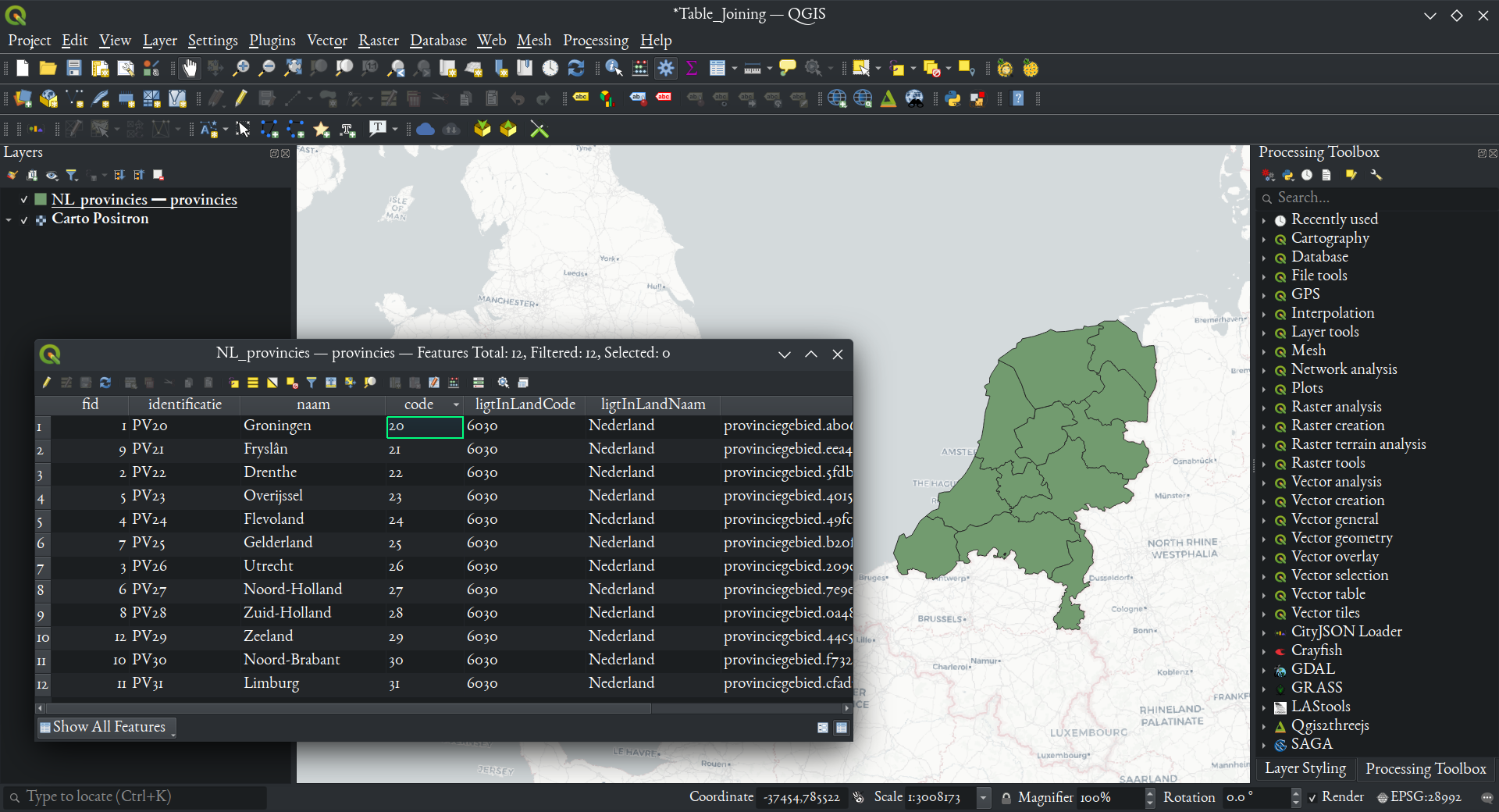
Below, we see a geopackage file of the provinces on The Netherlands (exported from the WFS service provided by PDOK here) loaded into QGIS, with the attribute table opened. Note that each of the 12 provinces has a unique "code" in the 4th column, which we'll use for a join.
In this CSV file, named SomeNumbers.csv, we've got a table of random, fictional numbers that we'll join to the provinces Geopackage file in QGIS. The table looks like this:
| ProvCode | SomeNumber |
|---|---|
| 20 | 679 |
| 21 | 432 |
| 22 | 221 |
| 23 | 689 |
| 24 | 843 |
| 29 | 356 |
| 30 | 812 |
| 31 | 121 |
| 41 | 585 |
Note that the above table doesn't contain some of the provinces (25 through 28), and it contains a fictional one (41).
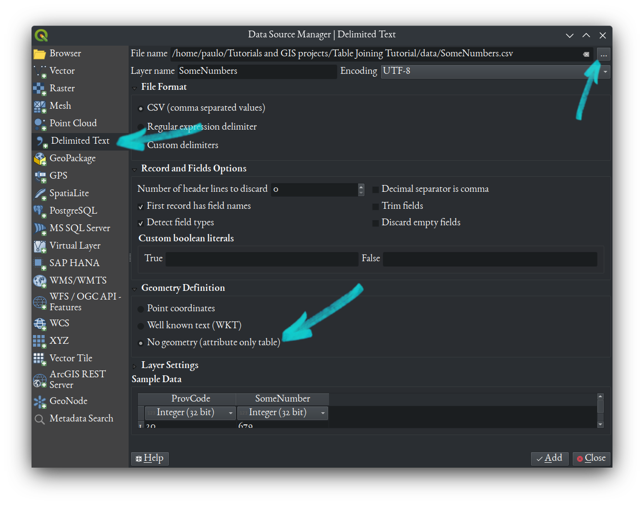
First, add that CSV file to the QGIS project using the Data Source Manager (click on  , or use shortcut: Ctrl+L), setting it as a non geometric data source:
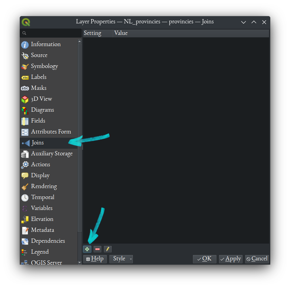
Then, open the Properties of the provinces layer, select Joins, and click the little + symbol at bottom to add a join:
That opens a window where we define the join. In that window, set the join layer to SomeNumbers, join field (equivalent to the foreign key) to ProvCode, and the target field (equivalent to the primary key) to code, as you see below:
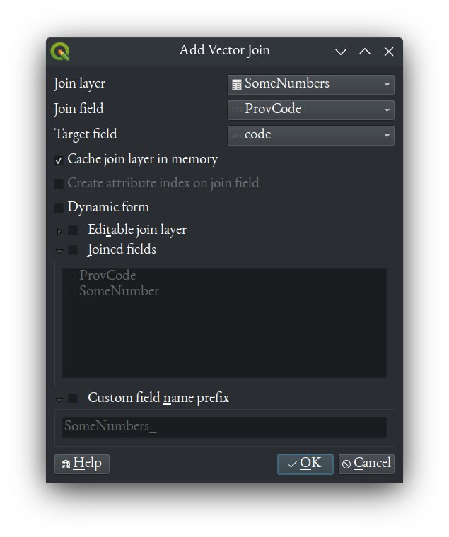
Then hit OK.
Back in the main QGIS window, if you look at the attribute table of the provinces layer, you'll see a left join has been performed, with NULL values in rows of the table where SomeNumbers has no match, and no record for the fictional province 41, which didn't find a match in the vector layer:
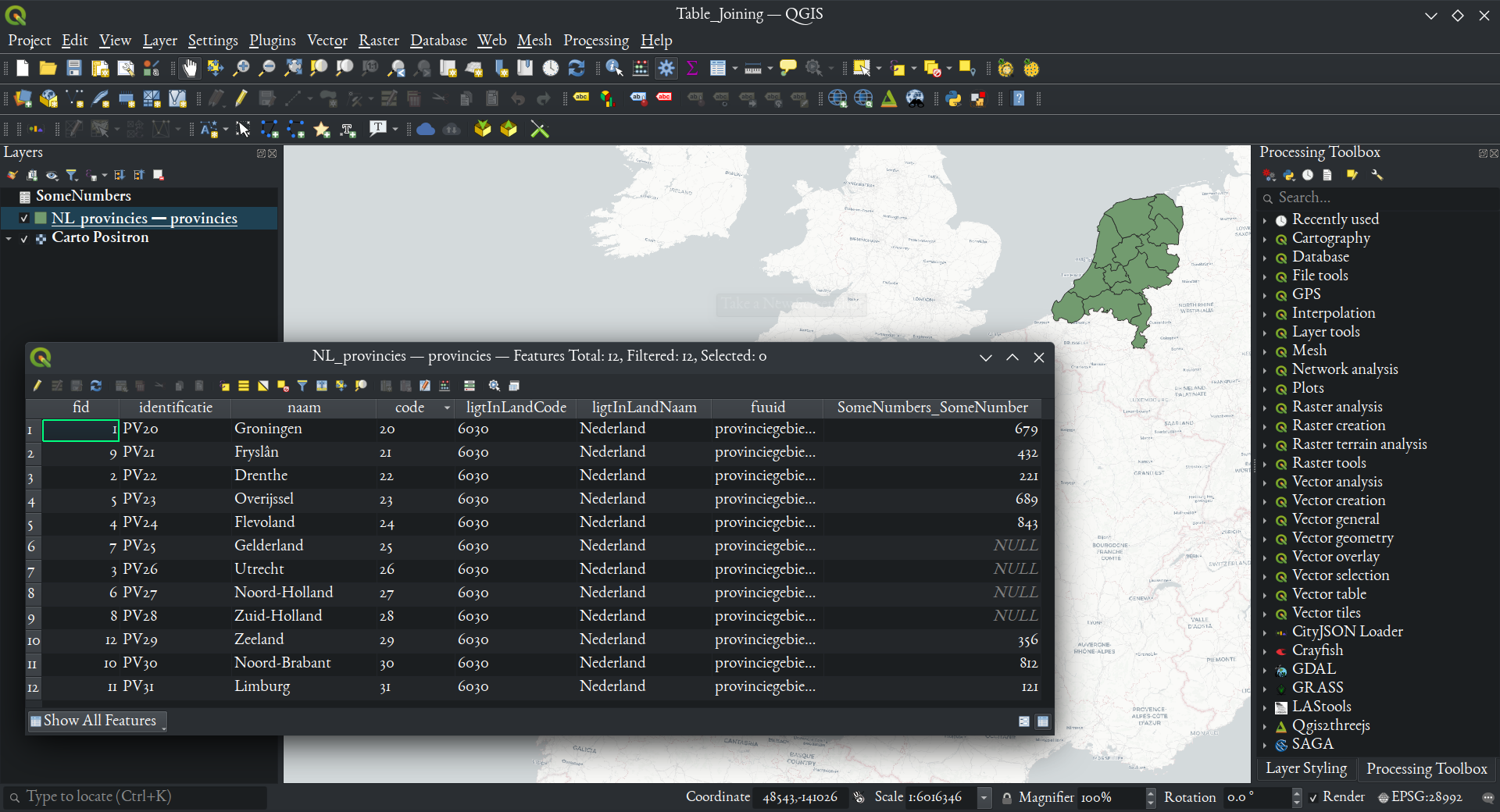
Remember, this doesn't change the underlying data file driving the layer (in this case the geopackage file), but you could export the layer once the join has been defined to a new file that will have the full, joined table as it's own.
QGIS Joins Producing New Data Files
Another way to join tables in QGIS is to use the "Join Attributes By Field Value" tool, available in the Processing Toolbox. This tool is a little more sophisticated in that it offers more options on how the join takes place. It also creates a whole new vector data file containing all the records of the table join, rather than defining the join "on the fly" in the QGIS project. Beyond performing a left join like the method described above, this tool also allows you to perform an inner join, by optionally discarding records from the left table that didn't find a match (see the "Discard records which could not be joined" option in the screen capture below). You can even save non-matching records from the left table as their own output data set, in case you need to analytically consider these at a later step in your work. Another benefit of using this tool is that it's Python scriptable, as are all the Processing tools in QGIS (type processing.algorithmHelp("native:joinattributestable") into the Python Console to see what input arguments are needed, and see this on how to call the tool in the console or your own scripts).
Here's what the tool looks like in the graphical user interface as we make an inner join by discarding non-matching rows:
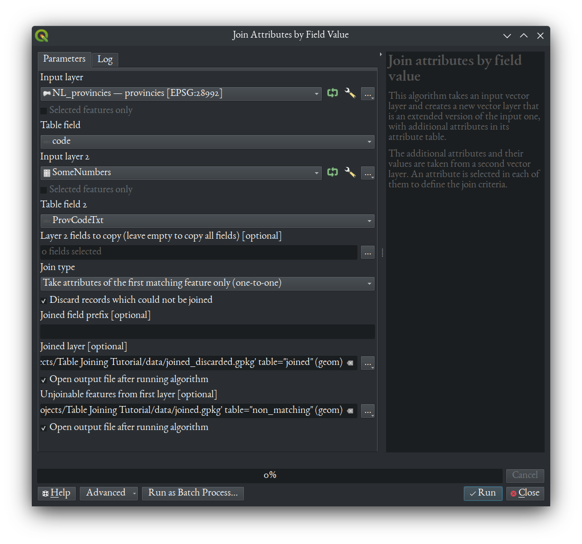
Note that for this tool, the data types of each field used have to match (e.g., a text field in the first table must match to a text field in the second table, not a numerical field). If that's not the case in your data already, you may have to create a new field of the matching data type in one of your tables and copy data from the existing field into it. This is fairly common when numerical code data (e.g., numerical digits for a country province ID) is treated by the software using it as quantitative data, when in fact it's nominal data that should not have math performed on it.