Back to main site

Vector Analysis for Wind Turbine Site Suitability

Paulo Raposo
Assistant Professor of Geovisualization
GIP Department, Faculty ITC, University of Twente
p.raposo@utwente.nl

2021-10-05. Revised 2022-09-25, 2023-09-05, 2023-09-12.

© Paulo Raposo, 2021. Free to share and use under Creative Commons Attribution 4.0 International license (CC BY 4.0).

Note: For a tutorial similar in theme to this one, but using different software, data, and analyses, see this one by Joseph Kerski for the ArcGIS platform.

Introduction

In this tutorial, we’ll use some fundamental GIS vector analysis tools to conduct a site suitability analysis, finding areas that satisfy a number of criteria. We’ll use publicly-available Dutch data. Topics covered include:

• using WFS and WMS data services,
• buffering,
• querying,
• dissolving,
• intersecting, and
• digitizing points from a CSV file.

Installing the software

We’ll need only QGIS 3.

Note that many of the data sources we’ll use will be online, so you’ll need a fairly good Internet connection.

Wind turbine placement in the Netherlands

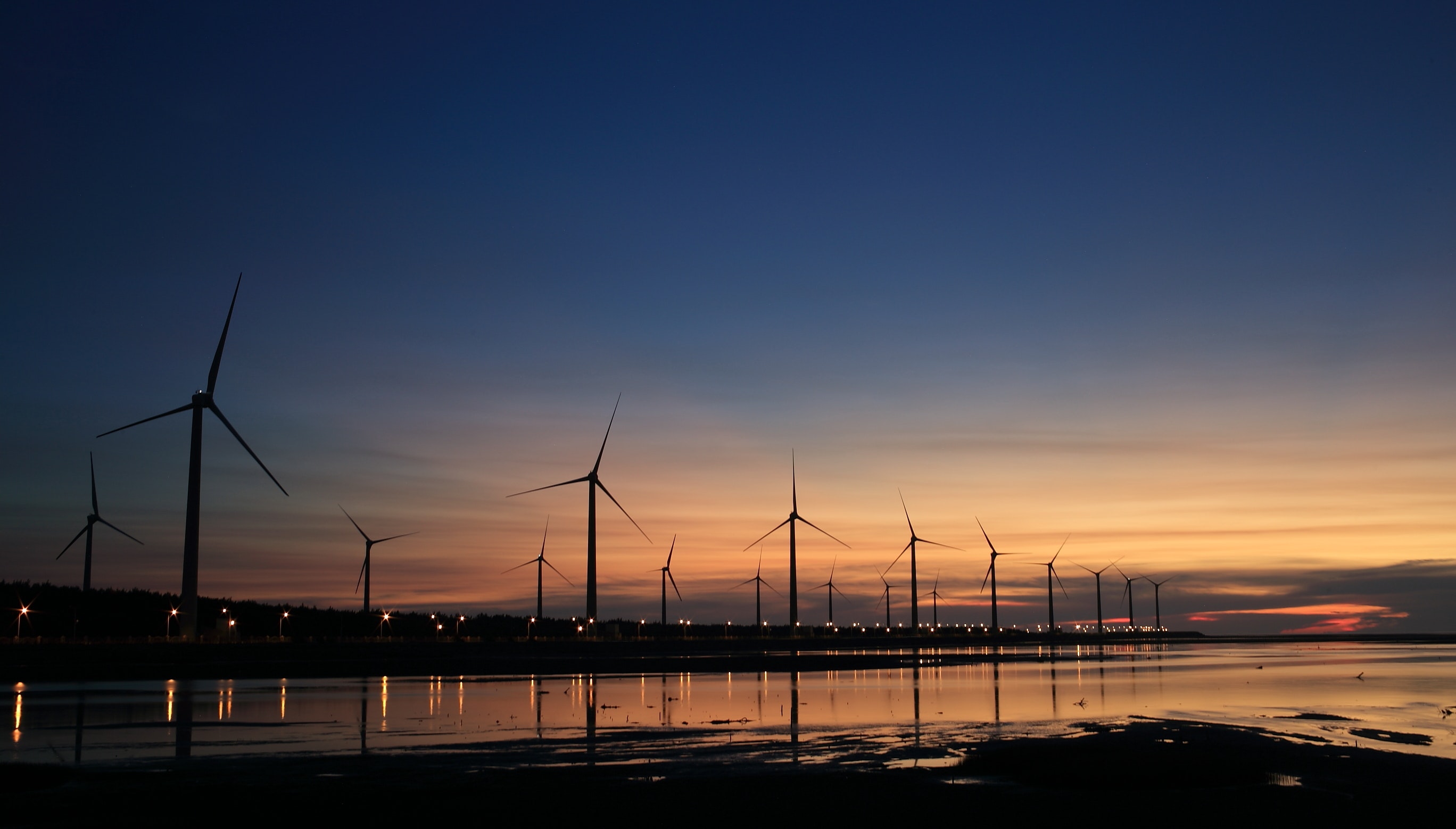
(photo credit: Flickr, via Pexels.com)

Wind turbines for generating electricity are becoming an increasingly critical part of electrical energy generation systems. Their placement matters: certain places simply experience more usable wind than others, installation and maintenance is easier done at certain locations and under certain conditions, ecological impacts on the surrounding environment differ by location, and public sentiment about having turbines within viewing or hearing distance can vary. So when governments or companies are considering installing turbines, several criteria are considered before deciding on installation sites. In this tutorial, we’ll simulate this situation, and try to find sites for new turbine installation in the Netherlands.

We’ll begin by looking for sites in the Netherlands that:

• are within a municipality that has at least 20,000 residents;
• experience a wind power potential of class 4 or higher;
• are at least 300 meters away from an existing turbine, but within 10 km of one.

Create and configure the QGIS project

Start up QGIS, and right away let’s make sure the coordinate system of our project gives us the ability to calculate accurate distances and directions. Under “Project,” go to “Properties.” Under “CRS” (coordinate reference system), search for “28992” in order to find the Amersfoort / RD New coordinate system, which provides planimetric accuracy for the Netherlands. Select it and click “OK.”

Save the project (a .qgz file) to your computer.

Accessing data through a web feature service (WFS)

The data we’ll use is available online through various web feature services. A WFS is a common standard for serving vector geospatial data, being a particular set of protocols by which a computer can serve GIS-ready data to other computers on the internet. WFS data sources will provide a URL to connect to (and, optionally, are password protected). Accessing WFS services with QGIS is easy.

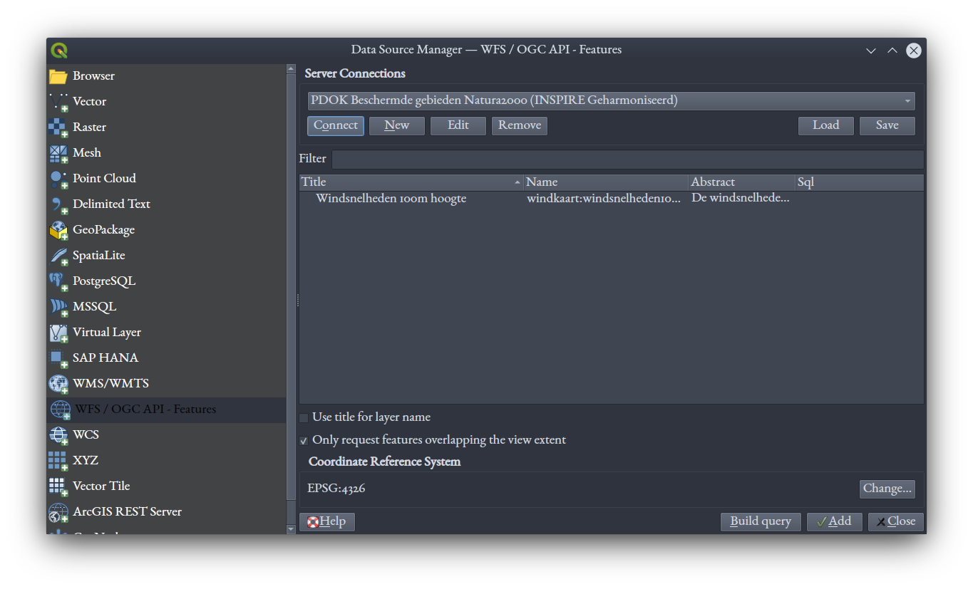
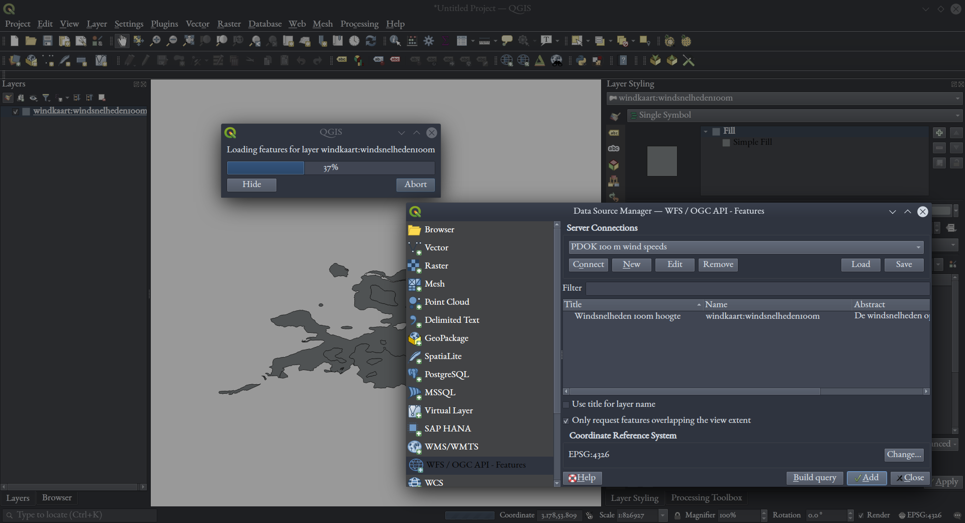
Open the “Data Source Manager” by clicking on the button, and select the “WFS / OGC API - Features” option on the left-most menu. You’ll be taken to the following dialog.

Click the “New” button near the top, to create a new connection to a WFS service (much like a contact in your address book). You’ll get the following dialog, where you simply name the connection something you’d like to find it by, and provide the URL of the service that the data provider has published on their website:

Edit 2023-09-05: Use this URL rather than the one you see in the image below: https://service.pdok.nl/rvo/windkaart/wfs/v1_0 (from PDOK).

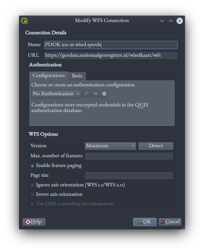
The above screenshot shows my connection details for the web service providing wind speed data that we’ll use shortly (the datasets and links to their webpages and WFS URLs are given in the next section of the tutorial).

Clicking “OK” will save the connection to your list of connections maintained by your local copy of QGIS.

To use this data source, back in the WFS section of the “Data Source Manager,” select your desired, pre-saved WFS service by name from the drop down menu and click the “Connect” button just below it. The table area below will update with available data layers provided by the WFS:

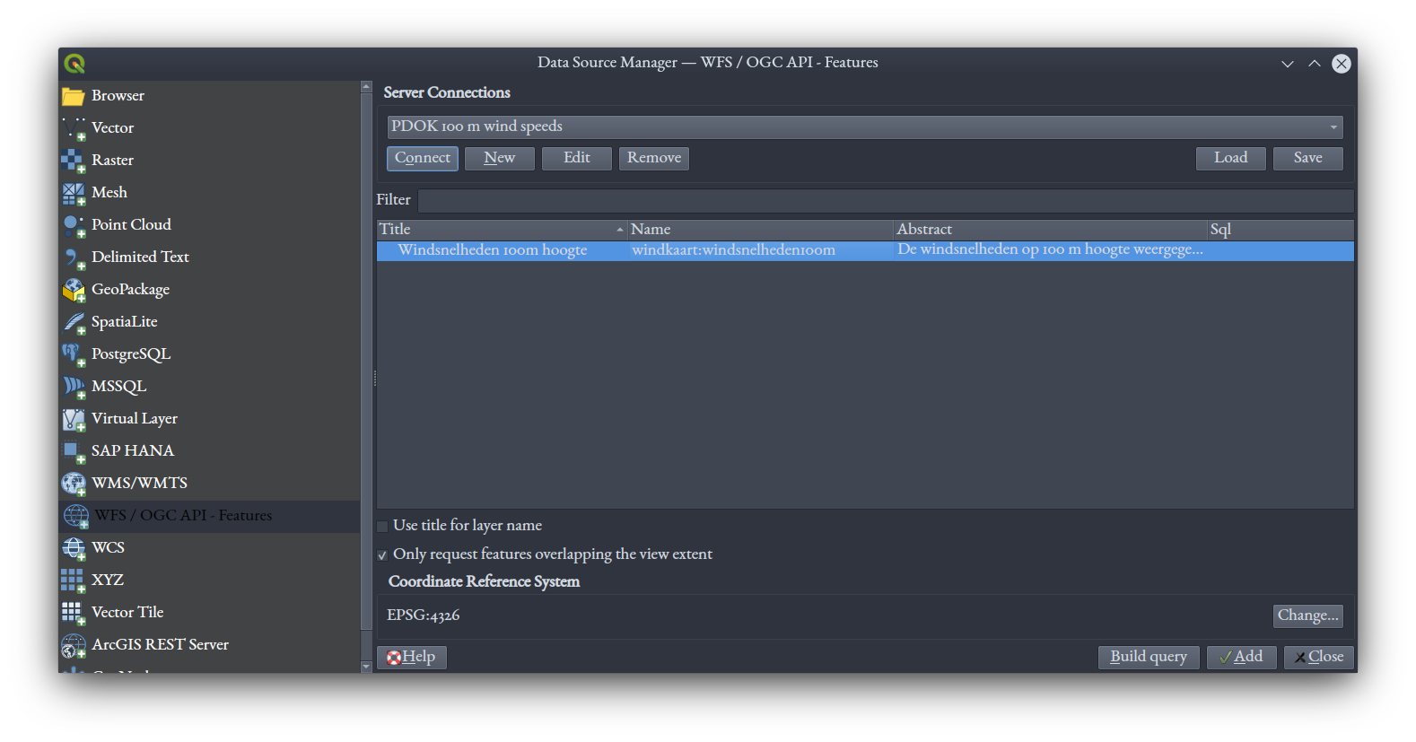
Select the layer you want to load by clicking and highlighting it (in the case of the wind speed data there’s only one, with the title “Windsnelheden 100m hoogte,” or “wind speed at 100 m height”). Uncheck the “Only request features overlapping the view extent” option near the bottom of the dialog. Click the “Add” button. QGIS will begin downloading that data layer and displaying it in the main window; depending on the size and your internet speed, it might take a little while:

Once they’re loaded, WFS data layers are like any other vector data layers in your GIS, with attribute tables and vectors you can symbolize.

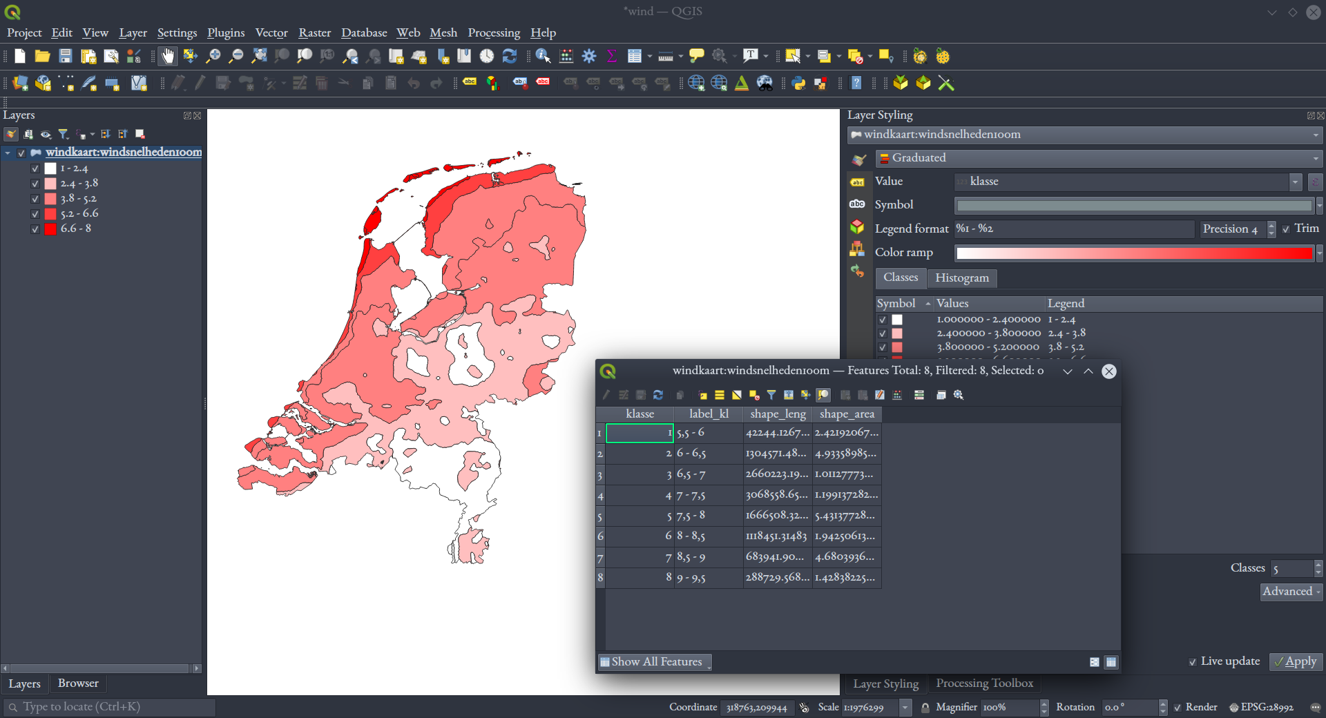
Note that QGIS continually asks and waits for WFS data over the web if you’ve loaded a WFS layer into your project, that this can cause a lot of delays in rendering. Turning layers off that you don’t need on will help, but so does saving a local copy of the data, so that you don’t have to continually get it from the online server. To do that, simply right-click the loaded layer in the “Layers” list and select “Export,” and “Save Features As.”

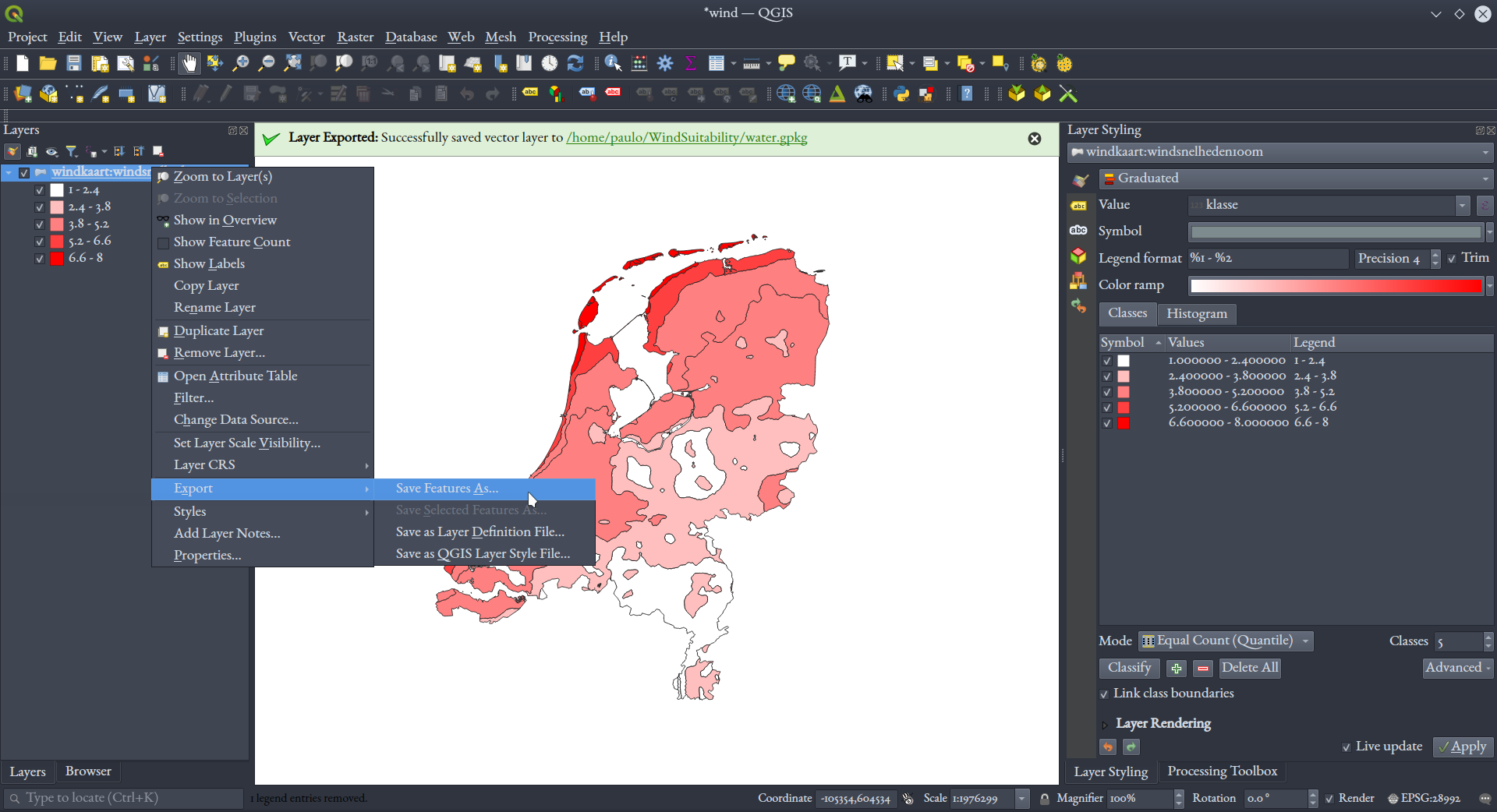
Then you can choose to save the layer to your own computer in various formats, like GeoPackage, Shapefile, or GeoJSON (and several others). You can also have data reprojected to another coordinate system than that provided by the WFS by specifying a “CRS” in this window – do that for your data layers in this tutorial, setting them to the same EPSG:28992 Amersfoort / RD New coordinate system we used for the project.

Using a local copy and removing the WFS layer from your project file will speed things up a lot by preventing web requests for the data every time you pan and zoom (and help with QGIS stability – save your project with Ctrl + S frequently!).

Adding a WMS layer

Web map services (WMS) are rather similar to WFS ones, except they serve raster data, and at various pixel resolutions depending on your project’s current cartographic scale (or “zoom” level). You can export the data to a local copy using the same “Layers” right-click option, and selecting a raster format like GeoTiff. Set the following WMS areal image service up in almost the same way as the WFS ones before, except in the “WMS / WMTS” section of the “Data Source Manager” window.

• Areal imagery
  • Choose either the “Actueel_ortho25” (25 cm pixels) or “Actueel_orthoHR” (8 cm) layer for the most current layer.

Compiling and analyzing the data

Now that we know how to access WFS services, let’s start collecting the Dutch data we’ll need. Begin by making WFS connections to the following three datasets, loading them into your project, and exporting local GeoPackage copies of them to work with:

• Locations of existing wind turbines.
• Average windspeeds at 100 m altitude.
• Districts and neighborhoods with accompanying census statistics, 2020.
  • Choose the “gemeenten2020” layer for municipalities.

Buffering

Let’s identify the areas 300 m around existing turbines by buffering those turbines. In the “Processing” window, search for “buffer,” and select the QGIS buffer too (there are other ones, like from GRASS and GDAL, but we’ll use the QGIS native tool). In the dialog that opens, select your turbines layer, specify 300 m, and check “Dissolve result.” Save your result to a GeoPackage, and give the layer a name when prompted.

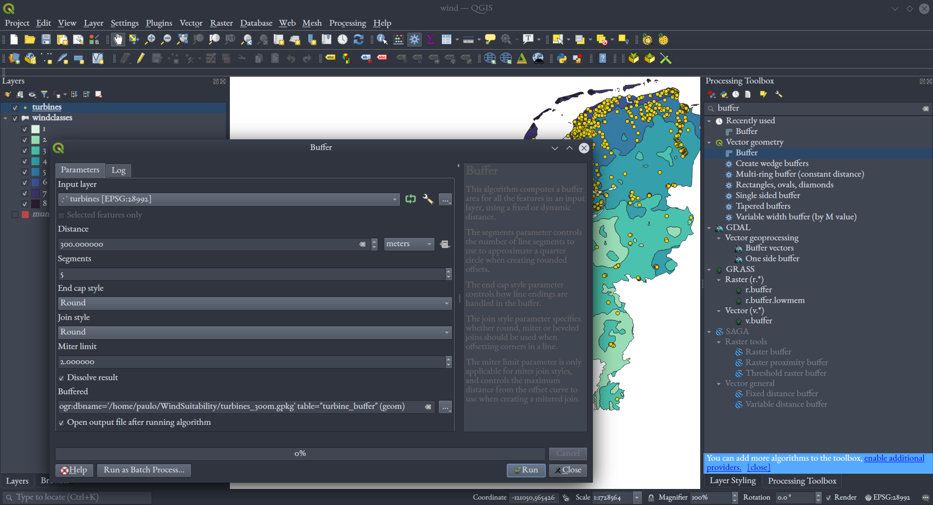
The tool should only take a few seconds. Once done, if you zoom in on an area with a lot of closely-packed turbines, you’ll see how we have polygons defining those dissolved buffers now.

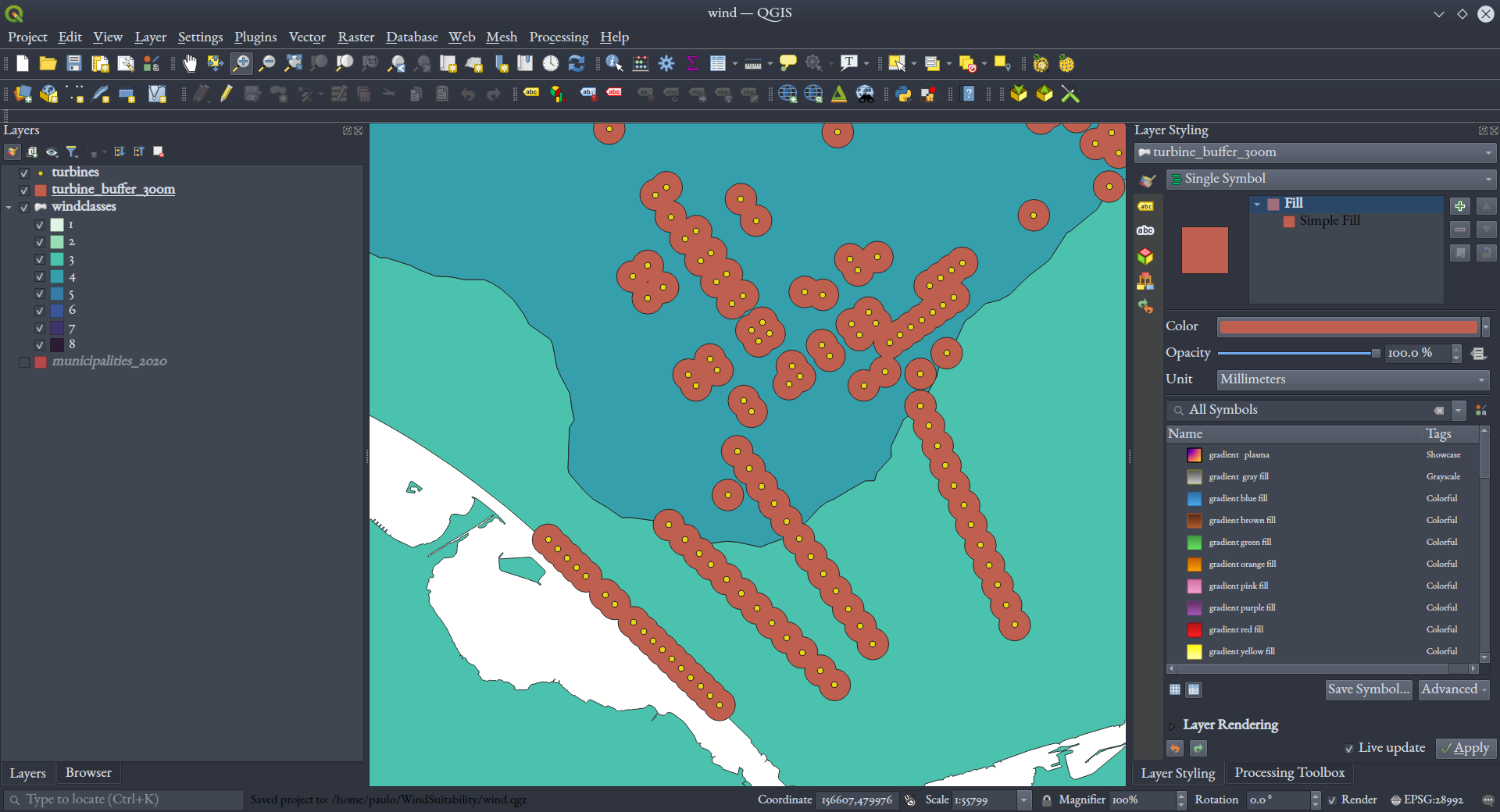
The area we defined above is where we don’t want turbines, but we also want them within 10 km of existing turbines. Make a buffer of 10 km around existing turbines, also dissolving the result. Below is a zoomed-in view of what our 300 m buffer looks like over our 10 km buffer.

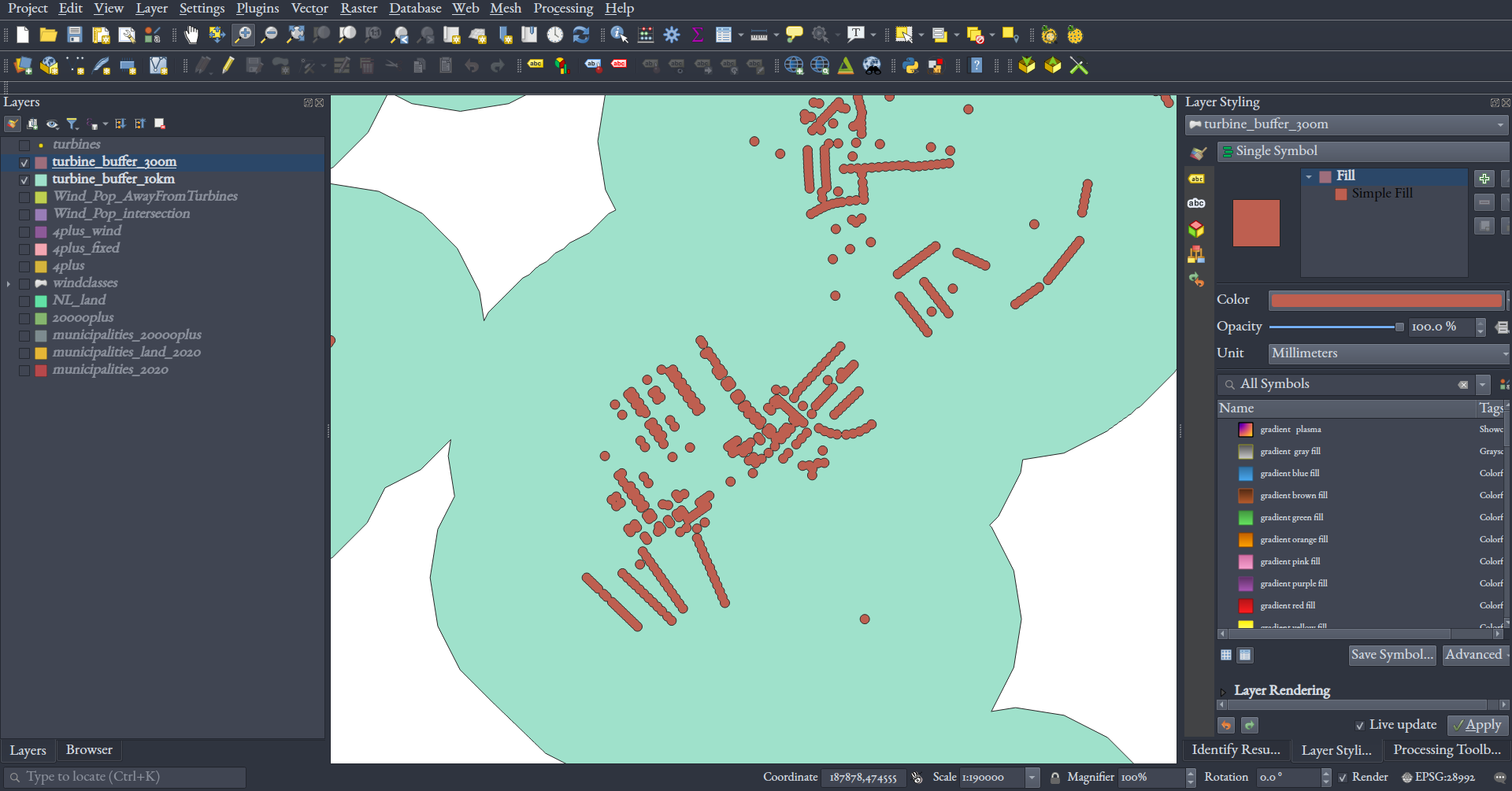
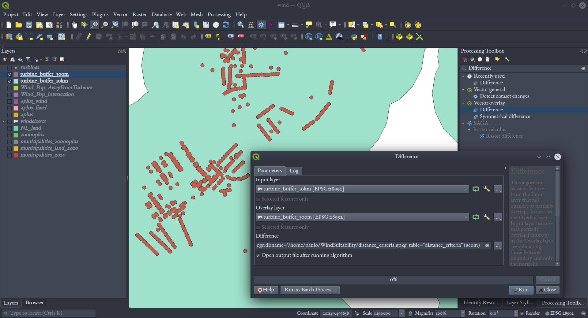
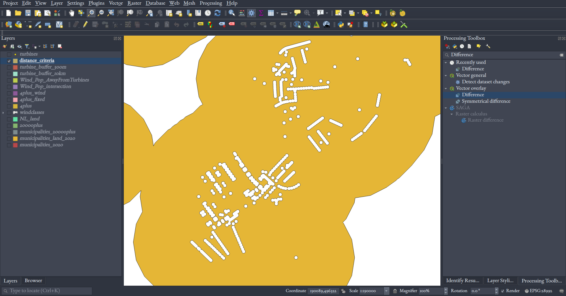
We want to cut the 30 m buffer areas out of the 10 km buffer area, since we don’t want to build turbines there. Do this with the “Difference” tool in QGIS, providing your 10 km buffers as the Input layer and your 300 m buffers as the Overlay layer to get a layer that looks like cookie dough with holes cut out:

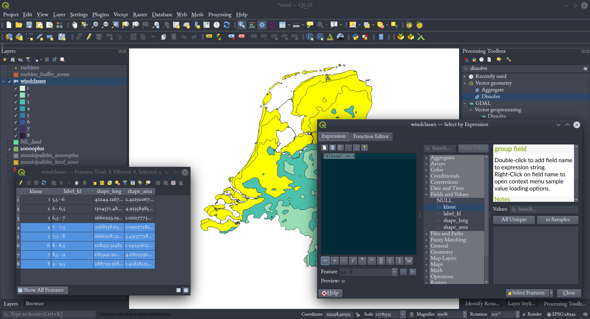
Querying

Have a look at the municipalities layer’s attribute table (right click on the layer in the “Layers” window). There’s a field there telling us whether each polygon is a water-filled area (i.e., the land belonging to a municipality, or waters under its jurisdiction).

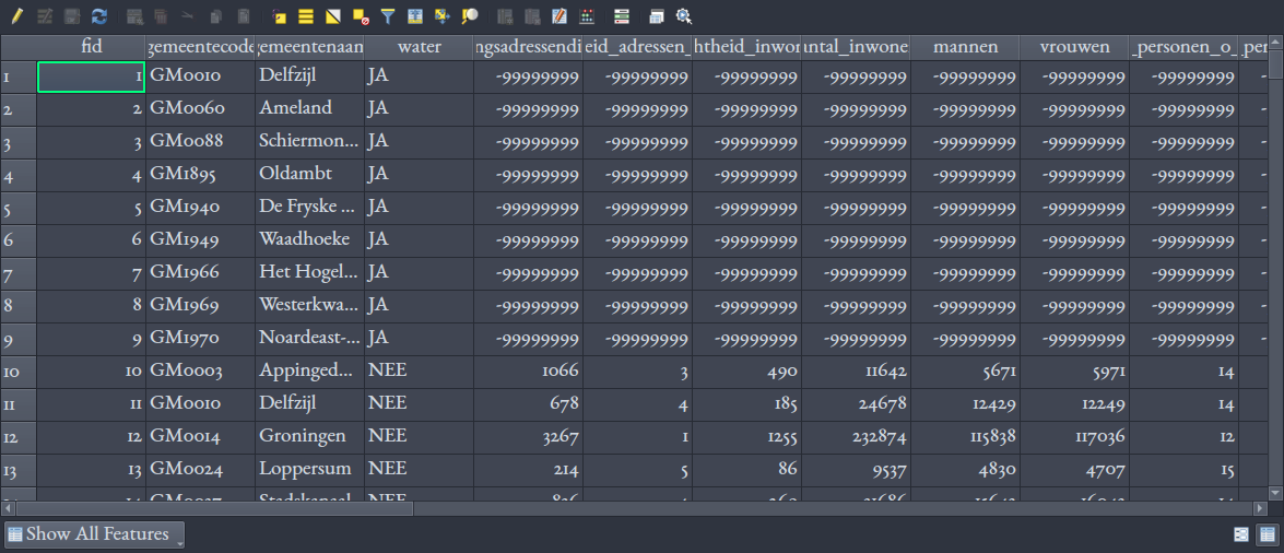
We’re only interested in potential on-land wind mills. Let’s select land-only municipality polygons. In the attribute table window, click the expression button, and write the following into the text area, to indicate that we want the field (in double-quotes) water to be equal to the string value (in single-quotes) NEE (for “no”):

"water" = 'NEE'

Then click the “Select Features” button, and notice how certain polygons on the map become highlighted.

Close the attribute table and query windows, and in the main window, right-click the municipalities layer and export it to a new layer, this time being careful to have the “Save only selected features” option checked.

We want to find municipalities where the population is at least 20,000. In the attribute table of your on-shore municipal polygons, build another expression to select for just that on the “aantal_inwoners” (“total residents”) field:

"aantal_inwoners" >= 20000

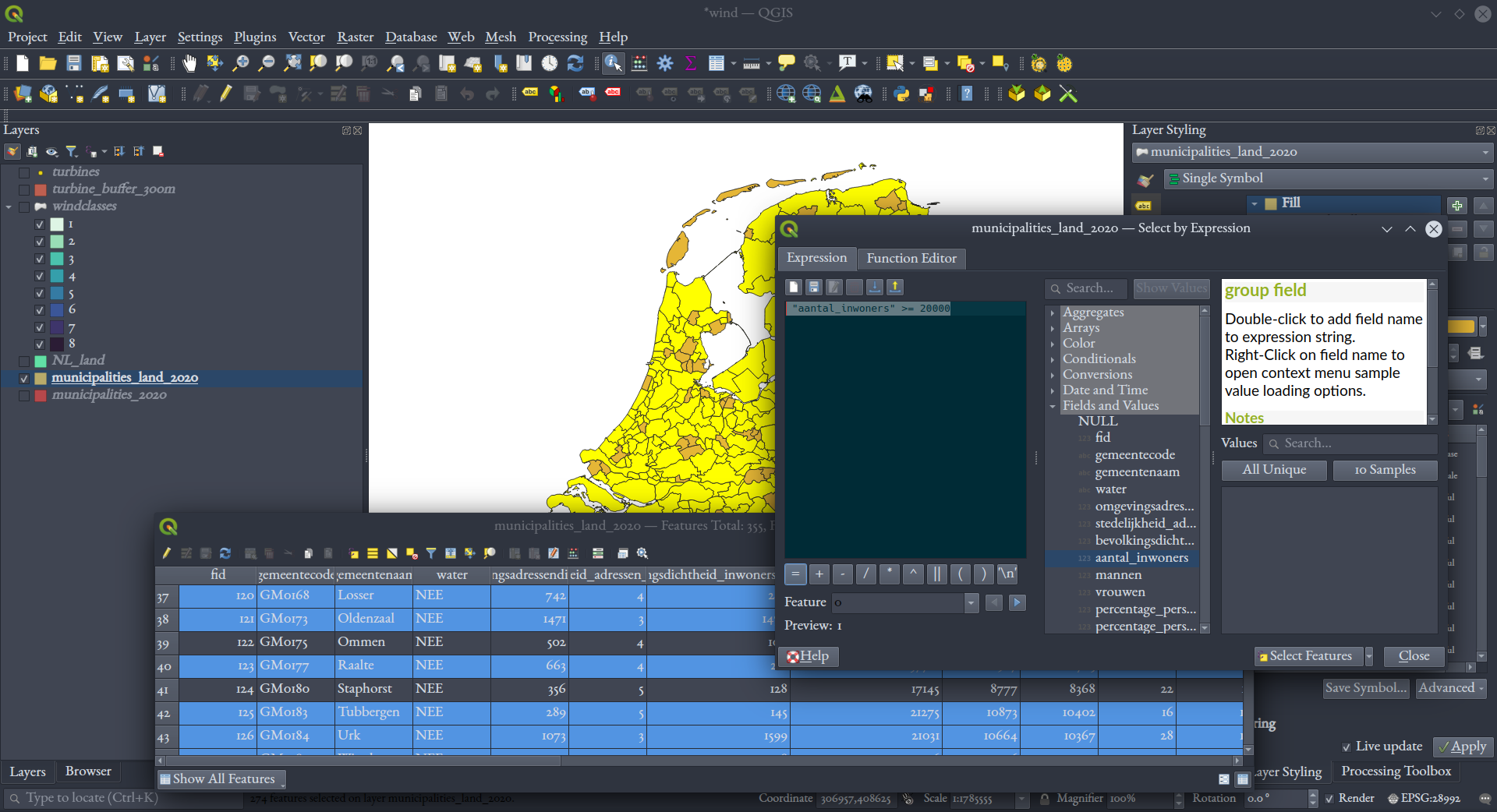
Save that layer to it’s own GeoPackage, again being careful to export only selected records. You should get an output like this:

We want areas with wind category 4 or higher, so we do the same query, select, and export-the-selected process on our wind speed data:

"klasse" >= 4

Dissolving

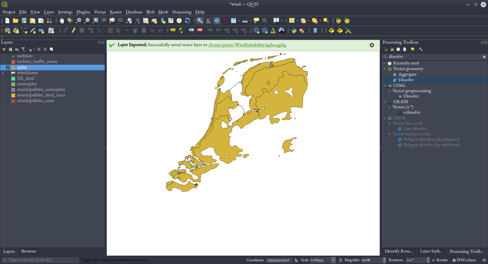
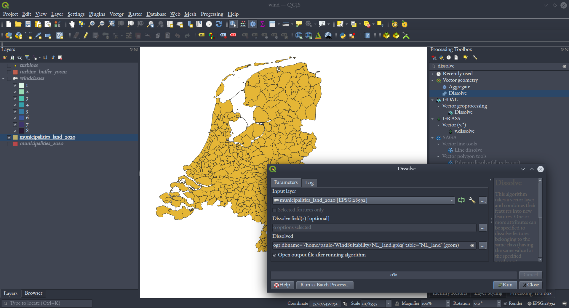
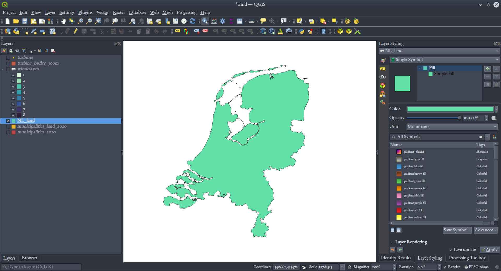
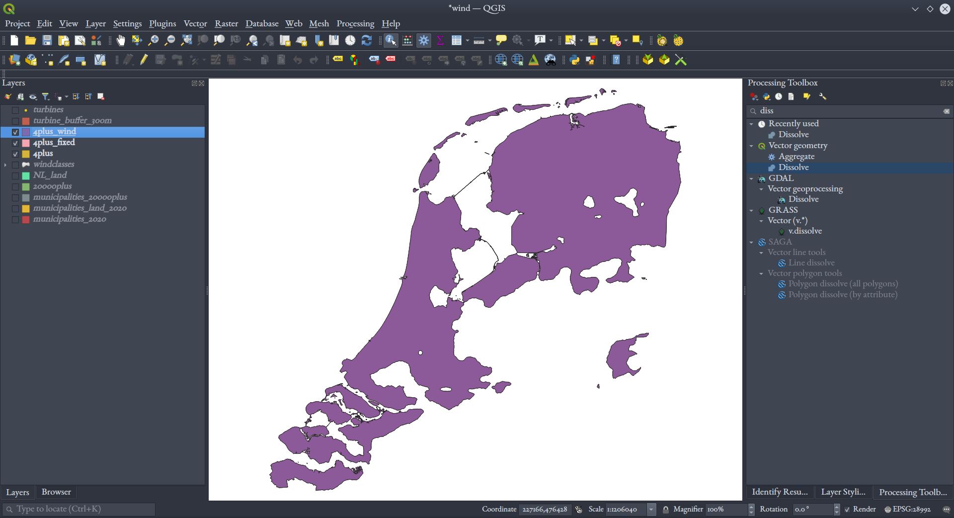
To get an unbroken polygon for all of the land areas of the Netherlands, let’s dissolve the on-shore municipalities data we just exported (not the layer with only populations above 20,000). Find the QGIS native “Dissolve” tool in the “Processing” window, and dissolve your layer without specifying a field to find matches on, again saving to a GeoPackage output with a name like “NL_land.”

Note: We could have gotten a very similar layer by dissolving the wind class data, too.

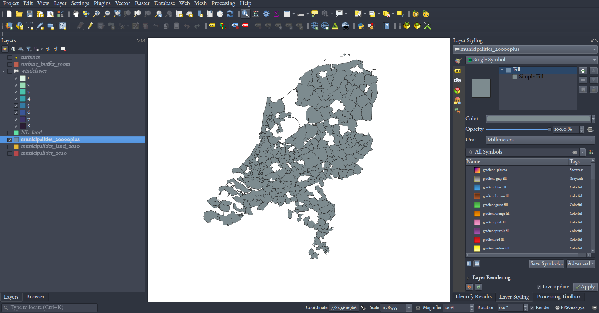
Do the same on the layer you created above with only municipalities of 20,000 or more, so that those all become contiguous areas:

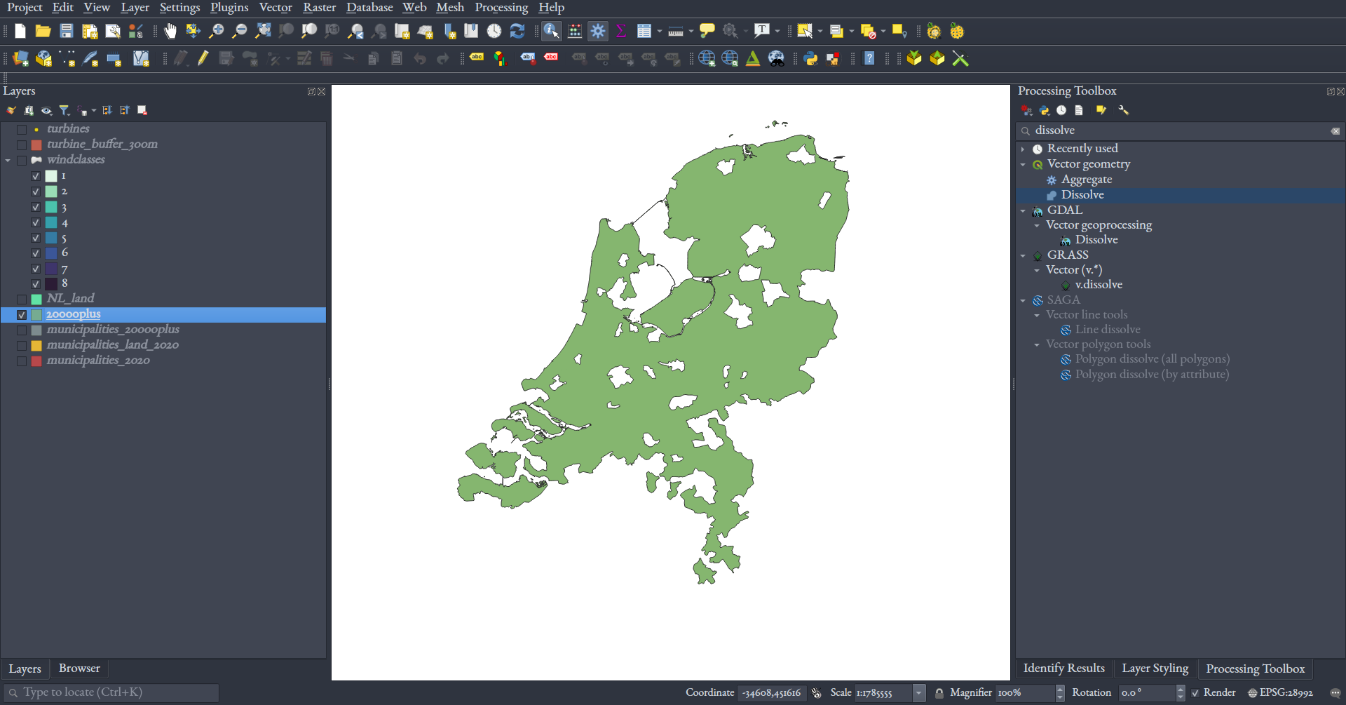
And do the same again with the 4 or higher wind classes.

Note: You may have to “fix geometries” (i.e., enforce data standard conventions about how the polygon data is saved) before this dissolve operation can work on the exported wind speed polygons – I did. If so, use the “Fix geometries” tool from the “Processing” window on your exported wind polygons; it doesn’t need any parameters beyond the input layer; just save the output to disk, and perform the dissolve on that layer.

Intersecting

Now, we’ve got 3 polygon layers in our project that reflect the population, wind class, and distance criteria we started with.

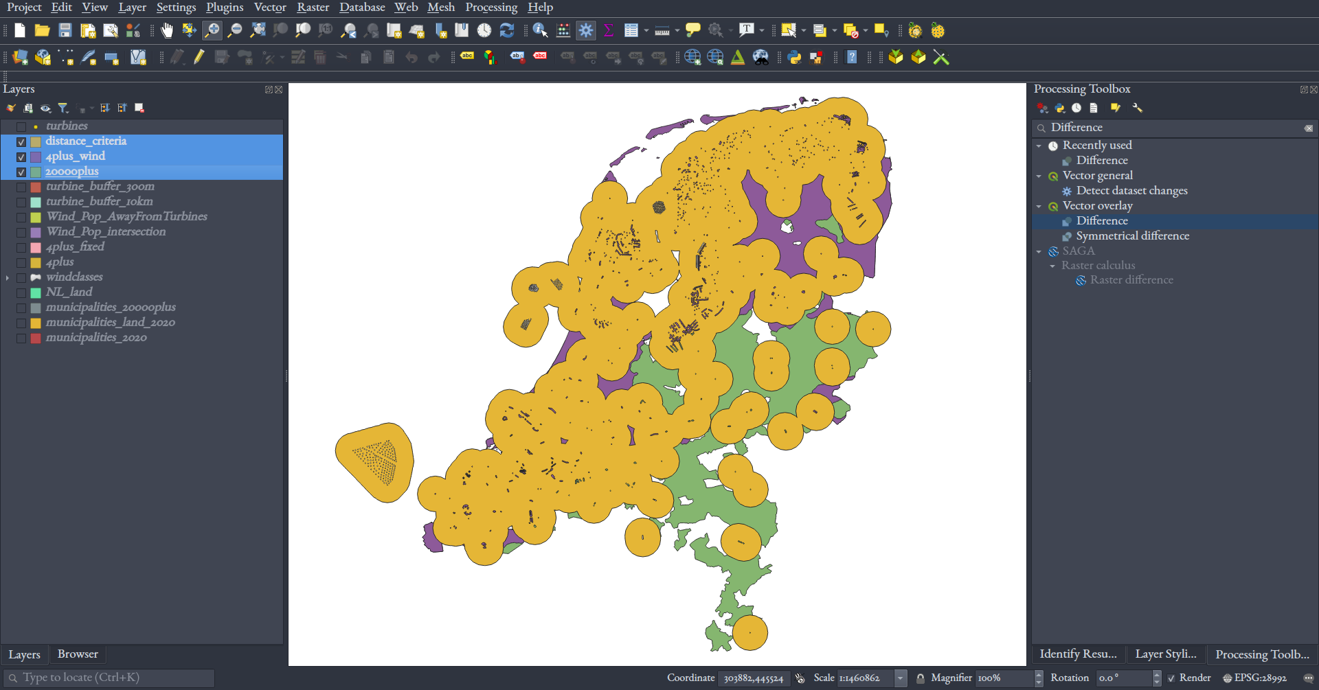
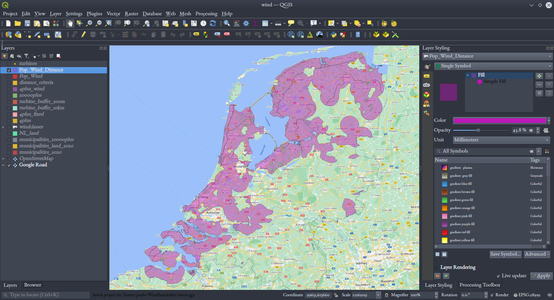
We need to find where all three of these intersect in order to find places where all three criteria are present. To do this, search for “Intersection” in the “Processing” window, because we’ll use that QGIS tool to make these intersections. The tool takes two layers at a time, one as “Input” and another as “Overlay.” First intersect any two of your three criteria polygon layers (e.g., the population and turbine buffer one), and then intersect their intersection product with the third criteria polygon. You should get this:

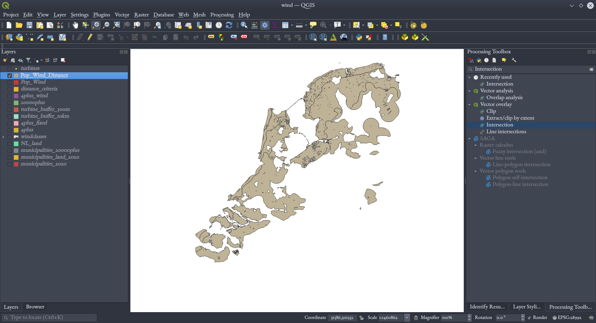
And we’ve now found all those areas that satisfy the three criteria we started with!

To give this visualization some context, let’s add a basemap layer. In the “Data Source Manager,” go to the “XYZ” section (for maps served as raster tiles), and click “New” to create a new connection to Google Maps. Name it “Google Road” and use the following URL:

https://mt1.google.com/vt/lyrs=m&x={x}&y={y}&z={z}

Click “Add” back in the “Data Source Manager,” and you’ll see that a layer of Google maps tiles has been added to the project. Drag it to the bottom of the layer stack, so your criteria vector polygons are on top. In the “Layer Styling” for your criteria overlay, set the opacity to around 50%.

The above has walked through an example of the basic process of conducting vector overlay, in this case applied to finding suitable sites. Our example has been realistic, but pretty drastically simplified, because there are many other things we would want to intersect with or avoid when building wind turbines in the real world. To name a few:

• buildings;
• roads;
• railways;
• water features;
• protected sites (historical, cultural, or ecological, or parks).

Still, let’s say we’ve found a place we’d like to add one turbine within the areas that satisfy our criteria – go ahead and pick a spot. We’ll find coordinates for that spot and digitize it for mapping in the next steps.

Digitizing a point from known coordinates using a CSV

To get the coordinate of any point under your mouse pointer in QGIS, right-click on that point:

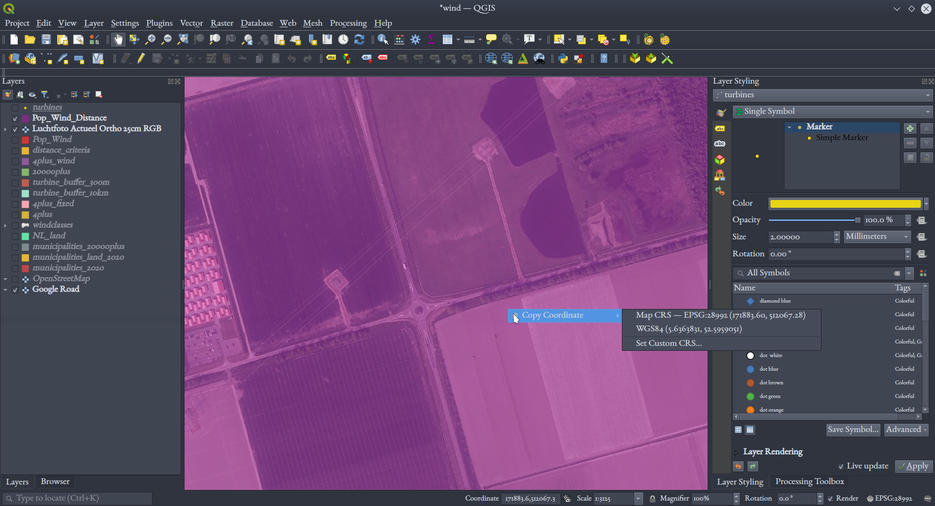
Copy the WGS84 coordinates.

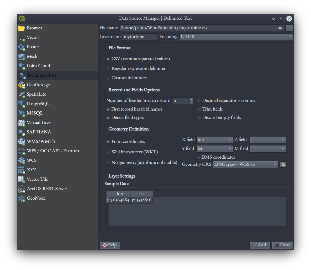
Next, open a basic text editor (I recommend Visual Studio Code, and not Windows' Notepad), and write the following into a new file, where the second line is the only data row, pasted from your clipboard:

lon,lat,label
5.6363831,52.5959051,"New turbine"

Save this as as CSV file (e.g., myturbine.csv).

Next, in QGIS, go to the “Data Source Manager,” and into the “Delimited Text” area. There, indicate your saved CSV file as the one to load, and ensure that other settings are as you see below, including the CRS of your CSV data being set to WGS84, and the X field set to “lon” and Y field to “lat.”

Click “Add” and close the “Data Source Manager.” You’ll see that your point has been added to the map:

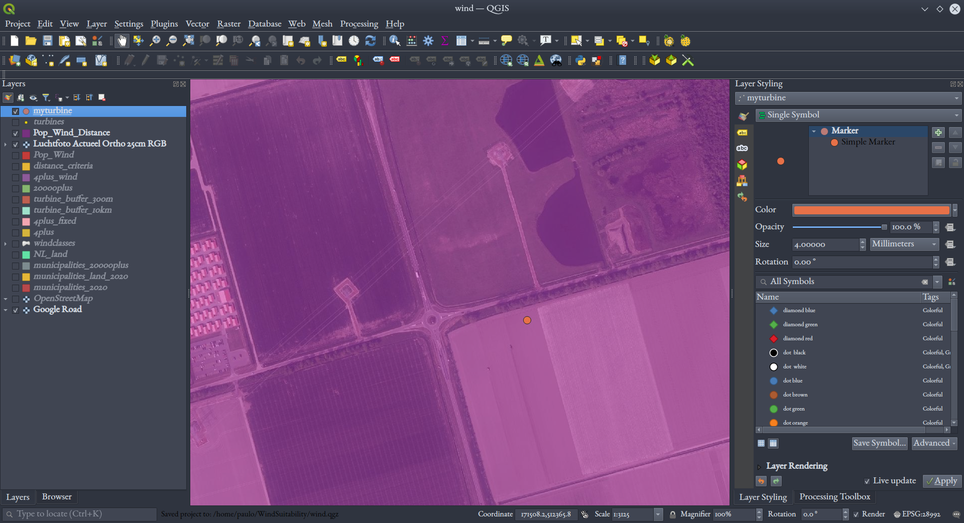
Right-clicking on the layer and opening the attribute table, you’ll see that it’s got only the two attributes you defined, lon, lat, and label.

Note: More attribute fields and data records could have been defined in our CSV before we imported it, if we wanted multiple points.

As a layer in the QGIS project, this can now be exported to a more sophisticated geospatial data format, like GeoPackage, in the same way we saw before.

(photo credit: Pixabay, via Pexels.com)